Forecasting Time Series Data Using Splunk Machine Learning Toolkit – Part II
Part II of the Forecasting Time Series blog provides a step by step guide for fitting an ARIMA model using Splunk’s Machine Learning Toolkit. ARIMA models can be used in a variety of business use cases. Here are a few examples of where we can use them:
- Detecting anomalies and their impact on the data
- Predicting seasonal patterns in sales/revenue
- Streamline short-term forecasting by determine confidence intervals
From Part 1 of the blog series, we identified how you can use Kalman Filter for forecasting. The observation we made from the resulting graphs demonstrated how it was also useful in reducing/filtering noise (which is how it gets its name ‘Filter’) . On the other hand ARIMA belongs to a different class of models. In comparison to a Kalman filter, ARIMA models works on data that has moving averages over time or where the value of a data point is linearly depending on its previous value(s). In these two scenarios it makes more sense to use ARIMA over Kalman Filter. However good judgement, understanding of the data-set and objective of forecasting should always be the primary method of determining the algorithm.
Objective
Part II of this blog series aims to familiarize a Splunk user using the MLTK Assistant for forecasting their time series data, particularly with the ARIMA option. This blog is intended as a guide in determining the parameters and steps to utilize ARIMA for your data. In fact, it is a generalized template that can be used with any processed data to forecasting with ARIMA in Splunk’s MLTK. An advantage of using Splunk for forecasting is its benefit in observing the raw data side by side with the predicted data and once the analysis is complete, a user can create alerts or other actions based on a future prediction. We will talk more about creating alerts based on predicted or forecasted data in a future blog (see what I predicted there ;)?)
If you have read part I of our blog, we will reuse the same dataset process_time.csv for this part. If not, click here to navigate to part I to understand the dataset.
Fundamental Concept for ARIMA Forecasting
A fundamental concept to understand before we move ahead with ARIMA is that the model works best with stationary data. Stationary data has a constant trend that does not change overtime. The average value is also independent of time as another characteristic of stationary data.
A simple example of non-stationary data is are the two graphs below, the first without a trendline, the second with a yellow trendline to show an average increase in the value of our data points. The data needs to be transformed into stationary data to remove the increasing trend.


Using Splunk’s autoregress command we can apply differencing to our data. The results are immediately visible through line chart visual! The below command can be used on any time series data set to demonstrate differencing.
… | autoregress value | eval new_value=value-value_p1 | fields _time new_value
Without creating a trendline for the below graph we can see that the data fluctuates around a constant mean value of ‘0’, we can say that differencing is applied. Differencing to make the data stationary can increase the accuracy and fit of our ARIMA forecast. To read more about differencing and other rules that apply on ARIMA, navigate to the Duke URL provided in the useful link section:

Differencing is simply subtracting the current and previous data points. In our example we are only applying differencing by an order of 1, meaning we will subtract the present data point by one data point in reverse chronological order. There are different types of non-stationary graphs, which require in-depth domain knowledge of ARIMA, however we simplify it in this blog and use differencing to remove the non-constant trend in this example 😊!
From part 1 of this blog series we can see that our data does not have a constant trend, as a result we apply differencing to our dataset. The step to apply differencing from the MLTK Assistant is detailed in the ‘Determining Starting Points’ section. Differencing in ARIMA allows the user to see spikes or drops (outliers) in a different perspective in comparison to Kalman Filter.
Walkthrough of MLTK Assistant for ARIMA
ARIMA is a popular and robust method of forecasting long-term data. From blog 1 we can describe Kalman Filter’s forecasting capabilities as extending the existing pattern/spikes, sort of a copy-paste method which may be advantageous when forecasting short-term data. ARIMA has an advantage in predicting data points when the we are uncertain about the future trend of the data points in the long-term. Now that we have got you excited about ARIMA, lets see how we can use it in Splunk’s MLTK!
We use the Machine Learning Toolkit Assistant for forecasting timeseries data in Splunk. Navigate to the Forecast Time Series Assistant page (Under the Classic Menu option) and use the Splunk ‘inputlookup’ command to view the process_time.csv file.
|inputlookup process_time.csv
Once we add the dataset click on Algorithm and select ‘ARIMA’ (Autoregressive Integrated Moving Average), and ‘value’ as your field to forecast. You will notice that the ARIMA arguments will appear.
There are three arguments that make up the ARIMA model:
| Argument | Definition |
| AutoRegressive – p | Auto regressive (AR) component refers to the use of past values in the regression equation. Higher the value the more past terms you will use in the equation. This concept is also called ‘lags’. Another way of describing this concept is if the value your data point is depending on its previous value e.g process time right now will depend on the process time 30 seconds before (from our data set) |
| Integrated – d | The d represents the degrees of differencing as discussed in the previous section. This makes up the integrated component of the ARIMA model and is needed for the stationary assumption of the data. |
| Moving Average – q | Moving Average in ARIMA refers to the use of past errors in the equation. It is the use of lagging (like AR) but for the error terms. |
Determine Starting Points
Identify the Order of Differencing (d)
As a refresher, we utilized the same dataset we worked with in part 1 of the blog series regarding the Kalman filter. As I input my process_time.csv file in the assistant, I enter the future_timespan variable as 20 and the holdback as 20. I’ve kept the confidence interval as default value ‘95’. Once the argument values are populated click on ‘Forecast’ to see the resulting graphs.

As a note, my ARIMA arguments described above are ARIMA(0,0,0) which can represented as a mathematics function ARIMA(p,d,q), where p,d,q = 0. We use this functional representation of the variables frequently in this blog for consistently with generally used mathematical languages.

When we click on forecast, observe the line chart graph from the results that show. This above graph confirms that the data is non-stationary, we will apply differencing to make it stationary. We can accomplish this by increasing the value of our ‘d’ argument from ‘0’ to ‘1’ in the forecasting assistant and clicking on forecast again. This step is essential to meet one of the main criteria’s of using ARIMA discussed in the ‘Fundamental Concept for ARIMA’ section.
Identifying AR(p) and MA(q)
After we apply differencing to our data our next step is to determine the AR or MR terms that mitigate any auto correlation in our data. There are two popular methods of estimating the these two parameters. We will expand on one of the methods in this blog.
Method 1
The first method for estimating the value of ‘p’ and ‘q’ is to use the Akaiki Information Criteria (AIC) and the Baysian Information Criteria (BIC), however using them is outside the scope of the blog as we will use a different method from the MLTK given the tools we have at hand. For the curious mind, the following blog contains detailed information on AIC and BIC to determine our ‘p’ and ‘q’ values:
Method 2
After we have applied differencing to our time series data, we review the PCAF and the ACF plots to determine an order for AR(q) or MA(q). We will apply ARIMA(0,1,0) in our ARIMA MLTK assistant and then click on ‘Forecast’ to view the results of the graph. The below image shows the values that we entered in the assistant:

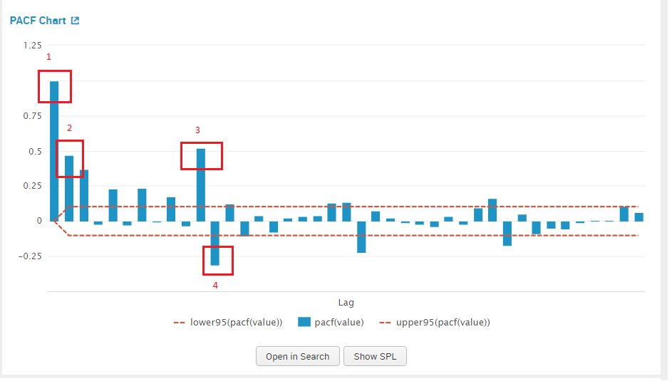
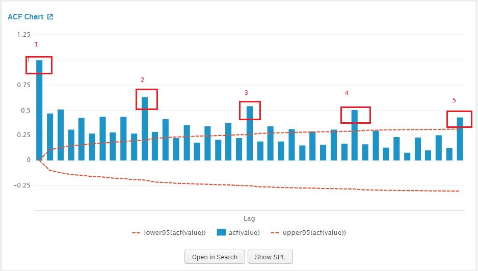
Once we click on forecast, we view the PACF plot to estimate a value for AR(p) model. Similarly we use the ACF plot to estimate a value for MA(q). The graphs are shown in the screenshot below.

We examine the PACF plot for a suggestion for our AR value, by counting the prominent high spikes. From the plot below I’ve circled the prominent spikes in the PACF graph. The value of AR (p) that we pick is 4.

We examine the ACF plot for a suggestion for our MA value, by counting the prominent high spikes. From the plot below I’ve circled the prominent spikes in the ACF graph. The value of AR (q) that we pick is 5.

We can now add in the values for the parameter integrated (d) – 1 and our estimates for AR – 4, and MA -5 in the Splunk MLTK. Once added in the assistant, click on ‘Forecast’.

For this particular combination for values we can see that once we click on ‘Forecast’, we get an error regarding the ‘invertability’ of the dataset as shown in the screenshot below. Without going too deep into the mathematics, it means that our model does not converge when it forecasts. I’ve added a link in the references and links section at the end for your interest! This error can be resolved by adjusting the values of model, similar to a ‘trail an error’ approach explained in the next section.

Optimize Your P and Q Values
Estimating this method of AR and MA is subjective to what can be considered as ‘prominent spikes’, this can result in estimating values of ‘q’ and ‘p’ that are not an optimal fit for the data. To resolve this we constructed a table displaying the R-squared and Root Mean Square Error (RMSE) values from the model error statistics from the MLTK assistance, for each combination of ‘p’ and ‘q’. An empty cell indicates an invertability error, while the other cells contain the value of R-squared and RMSE.
A higher R-squared indicates a better fit the model has on the data. R-squared is the amount of variability that the model can explain on the process time data points.
On the other hand, the lower the RMSE is the better the fit of the model. Root mean square is the difference between the data points the model predicted and our holdback points from the raw data.
We pick values of ‘p’ and ‘q’ that minimize RMSE and maximize R-square as the best fit to our data. From the table below we can see that q=5 and p=5 optimize the prediction for us.
| Integrated (d) = 0 | AutoRegressive (p) | ||||||
| 0 | 1 | 2 | 3 | 4 | 5 | ||
| Moving Average (q) | 0 | R2 Stat: -0.0015 RMSE: 19.31 | R2 Stat: 0.1976 RMSE: 16.35 | R2 Stat: 0.1977 RMSE: 16.34 | R2 Stat: 0.2699 RMSE: 15.60 | R2 Stat: 0.2696 RMSE: 15.60 | R2 Stat: 0.3114 RMSE: 15.14 |
| 1 | R2 Stat: 0.2401 RMSE: 15.91 | R2 Stat: 0.2486 RMSE: 15.82 | R2 Stat: 0.2780 RMSE: 15.51 | R2 Stat: 0.2329 RMSE: 15.98 | – | R2 Stat: 0.4053 RMSE: 14.07 | |
| 2 | R2 Stat: 0.2452 RMSE: 15.85 | – | – | R2 Stat: 0.3017 RMSE: 15.25 | R2 Stat: 0.3214 RMSE: 15.03 | – | |
| 3 | R2 Stat: 0.2872 RMSE: 15.41 | R2 Stat: 0.4185 RMSE: 13.92 | R2 Stat: 0.4428 RMSE: 13.62 | R2 Stat: RMSE: | R2 Stat: 0.4343 RMSE: 13.72 | R2 Stat: 0.4456 RMSE: 13.58 | |
| 4 | R2 Stat: 02826 RMSE: 15.46 | R2 Stat: 0.4185 RMSE: 13.92 | R2 Stat:0.3241 RMSE: 15.00 | – | – | – | |
| 5 | R2 Stat: 0.2826 RMSE: 15.46 | R2 Stat: 0.3133 RMSE: 15.99 | R2 Stat: 0.4385 RMSE: 13.67 | – | – | R2 Stat: 0.4515 RMSE: 13.52 |
Viewing Your Results
Once we have picked the values of p and q that optimize our model, we can go ahead plug the numbers in our assistant and click on forecast to display the forecasted graph. The values to plug in the assistant are as follows: p-5, d-1, q-5, holdback-20, forecast-20. The screenshots below show the values entered in the assistant and the resulting forecast graph.


A this point many would be satisfied with the forecast as the visual of the data itself is enough to analyse, asses and then make a judgement on the action(s) to take. The next step details how you can view the data and lists some ideas of alerts that can be constructed
Next Step
We can view the SPL used powering the graph by either clicking on ‘Open in Search’ or ‘ ‘Show SPL’. I prefer the ‘Open in Search’ option as it automatically open a new tab, allowing me to further understand how the SPL is constructed in the forecast and to view the data. Once a tab browser tab opens click on the ‘statistics’ option to view the raw data points, predicted data points and the confidence intervals created by our model. I have added the SPL from the image for your convenience below:
| inputlookup process_time.csv | fit ARIMA _time value holdback=20 conf_interval=95 order=5-1-5 forecast_k=40 as prediction | `forecastviz(40, 20, "value", 95)`

I added another filter to my SPL to only view the forecasted process data from the ARIMA model as shown below:
| inputlookup process_time.csv | fit ARIMA _time value holdback=20 conf_interval=95 order=5-1-5 forecast_k=40 as prediction | `forecastviz(40, 20, "value", 95)` | search "lower95(prediction)"=*

The resulting table lists all the necessary data in a clean tabular format (that we are all familiar with) for creating alerts based on our predicted process time. Here are some ideas on creating alerts based on the data we worked with:
- Create alert when the predicted value of the process time goes above a certain threshold
- Create alert when the average process time over a timespan is predict to stay above normal limits
- Create alert based on outlier detection, when the predicted data is outside the lower or upper boundaries
Creating alerts based on our predict data allows us to be proactive of potential increase or decrease of our input variable
Summarizing ARIMA Forecasting in MLTK
Lets summarize what we have discussed so far in this blog:
- A mathematical prerequisites of the model
- Determining differencing requirement
- Determine starting values for AR() and MA()
- Optimize your AR() and MA() values based on error statistics
- Forecast your data based on values decided in Step 4
- View data and determine any alerts conditions
Prior to the above steps, we need to ensure that our data has been pre-processed or transformed in a MLTK-friendly manner. The pre-process steps include but not limited to; ensuring no gaps in the time series data, determine the relevance of data to forecasting, group data in time intervals (30 second, 1 minute etc). The pre-processing steps are important to create uniformity in the data input allow Splunk’s MLTK to analyse and forecast your data.
Hopefully this blog, streamlines the process of forecasting using ARIMA in Splunk’s MLTK. There are limitations as with any algorithm on forecasting using this method, as it involves a more theoretical knowledge in mathematics I’ve added two links in the the useful links section (first link is navigates you to on ‘datascienceplus.com’ and the second to ’emeraldinsight.com’) to further read on them.
© Discovered Intelligence Inc., 2019. Unauthorised use and/or duplication of this material without express and written permission from this site’s owner is strictly prohibited. Excerpts and links may be used, provided that full and clear credit is given to Discovered Intelligence, with appropriate and specific direction (i.e. a linked URL) to this original content.


