Forecasting Time Series Data Using Splunk Machine Learning Toolkit – Part I
In this blog we will begin to show how Splunk and the Machine Learning Toolkit can be used with time series data, which is generally the most common type of data that is kept in Splunk!
Time series data are data points indexed sequentially at equally spaced intervals in time. In this blog series we will cover using Kalman Filter algorithms found in Splunk and Splunk’s Machine Learning Toolkit. Kalman are some of the many algorithms different that are provided by Splunk for forecasting.
A common and practical use of these algorithms is Splunk’s native ‘predict’ command. The ‘predict’ command utilizes variations of Kalman Filter algorithms which we will detail later in the blog. Some practical applications of forecasting time series data are in social platform data, financial data, system logs and application logs. In IT Ops, analyzing time series data we can yield actionable intelligence such as early detection of outliers and understanding short-term and impact/trends to name just a few.
Understanding the Dataset
Part I of the blog will focus on utilizing variations of the Kalman Filter for forecasting. My local machine’s “% Process Time” counter was onboarded using Splunk Windows TA to create the test dataset.
The process time data was formatted and processed to be ‘machine friendly’ by converting the time to epoch time and saving events in csv format for further analysis by users. The queries in this blog can be performed on live or raw data in your Splunk instance to achieve the same result for forecasting your raw data.
Before we begin our analysis, here are two concepts to help determining an algorithm for forecasting. Trend is the general direction a time series data is developing towards, it can be; downward, increasing, stationary or any combination of the three. Seasonality is a set of characteristics of time series data which shows predictable and repeated changes of data over a time frame.
The dataset shows the average process time in a 30 second window between 9:30-12:30pm on July 31st, 2018. I picked this time to determine the short-term impact on process time of my local machine executing automated scripts. We could have picked a daily-trend as opposed to a 30 second average window, however, selecting a time-frame depends on the requirements and scope of the question.
- process_time.csv (click to download)
To upload the dataset we navigate to settings-> lookups -> add new lookup table file as save as ‘process_time.csv’
Once the csv file has been uploaded, execute the below query in Search to view the data.
| inputlookup process_time.csv
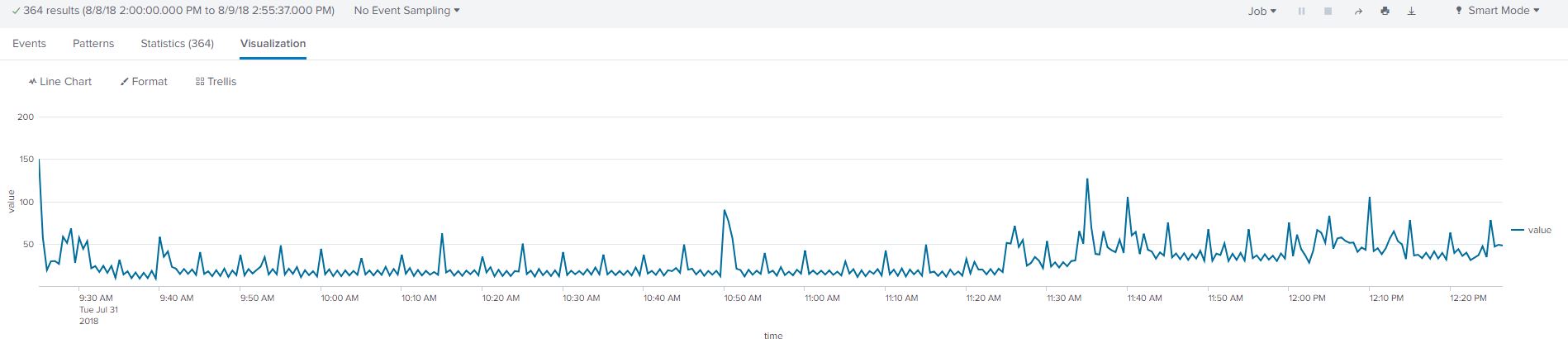
The query shows the data in a tabular format listing the execution time and the average processes time in 30 second intervals over a few hours. Click on the ‘Visualization’ tab and select ‘Line Chart’ as your visual. The resulting visual shows the data as a graph outlining the trend and seasonality of the data.
Splunk’s Native Predict Command
We will use Splunk’s ‘predict’ command which leverages variations of Kalman Filters. Detailed Information on the Splunk command, its parameters and examples can be found on this page:
https://docs.splunk.com/Documentation/Splunk/latest/SearchReference/Predict
This table below summarizes the algorithms available to use on time series data and their descriptions:
| Algorithm | Description |
| LL (Local Level) | A simple univariate time series algorithm requires a minimum 2 data points. It does not consider seasonality or trend and extends the time series graph by adding the gaussian noise. We will not delve deep into the mathematics of this algorithms. |
| LLT (Local Level Trend) | A univariate model that utilizes a trendline for forecasting. A trendline is a line of best fit and a minimum of 3 data points are required. |
| LLP (Seasonal Local level) | A univariate model that accounts for seasonality. Seasonality can be repeated and predictable events during time of day, daily, weekly or monthly etc. |
| LLP5 (Combines LLT and LLP) | A univariate model combining the weighted average of LLT (trend) and LLP (seasonality) to predict your time series data. It computes a default confidence interval of 95%, when selected. |
| LLB (BiVariate Local Level) | A bivariate model with no trends and seasonality requiring a minimum of 2 data points. It uses one field to predict the other field by calculating the correlation between the variables. This algorithm can be used to complete one missing field using correlation. As a result we can not use the future_timespan parameter to forecast both fields. |
| BiLL (BiVariate Local Level) | A bivariate mode predicts by calculating the covariance of the two variables to predict future events. |
We will only use univariate algorithms to forecast for simplicity and to demonstrate utilizing the Splunk functionality. In addition to the algorithms for Kalman Filter, some useful parameters for the predict command and their description are shown below:
| Argument | Description |
| future_timespan | Use this argument to specify how many future predictions you want the algorithm to compute. This argument must be a non-negative integer. Future_timespan is used in conjunction with the holdback argument below. |
| holdback | Use this argument to specify the split of data points not to be used by the predict command. E.g With 100 data points and a holdback value of 10, that would mean that the algorithm will learn from the first 90 data points only. The remaining 10 data points can be used for analyzing model accuracy. |
| period | Specifies the length of the time period for the seasonality to occur again. The algorithms LLP and LLP5 automatically attempt to calculate the period if no value is specified. |
| lowerXX | ‘XX’ Specifies the lower confidence interval for the prediction. The integer must be between 0 and 100 |
| upperYY | ‘YY’ specifies the upper confidence interval for the prediction. The integer must be between 0 and 100 |
Using SPL to Forecast
Now that we have some background on the options we can use with the predict command, lets see how we can leverage that in our search. As rule of thumb we should always use the ‘timechart’ command before using the ‘predict’ function, however the data in the lookup has already been statistically aggregated within 1-minute spans for ease of calculations.
| inputlookup process_time.csv | predict value algorithm=LL future_timespan=50
It’s obvious from the line chart that the result is not what we expect, the local level algorithm filters the fluctuation in our events as noise. This chart is does not give any useful information on our trend or seasonality in our data.
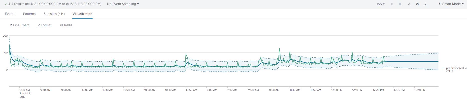
| inputlookup process_time.csv | predict value algorithm=LLP future_timespan=50

Utilizing the Local Level Trend algorithm, we see that there is a general downward trend of our process time. Like the previous algorithm, we are attempting to forecast the next 50 events. This method gives us the trend however, falls short of depicting recurring trends. The upper confidence intervals can be used to find the probability that the process time will next exceed by 95% of the time.
| inputlookup process_time.csv | predict value algorithm=LLP future_timespan=50

From the LLP algorithm we can see that the result is much better, it captures the ‘spikes’ in our data. The spikes can be explained by a program executing every 5 minutes on my local machine. The predicted events are however too similar in forecasting.
| inputlookup process_time.csv | predict value algorithm=LLP5 future_timespan=50
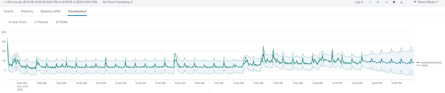
Now, by combining trend and seasonality we used the LLP5 algorithm. The resulting trend looks satisfactory as it accounts for the regular spikes at the 5-minute interval and the downward trend of the process time value. Now we would like to modify our holdback and confidence interval values. Instead of adjusting them in the Splunk Query, we will use the MLTK ‘Forecast Time Series’ Assistant as it provides some better interfaces to work with.
In MLTK version 3.3 and above we can find the assistant in Classic -> Assistants -> Forecast Time Series from the navigation bar. In MLTK version 3.2 we can find it in Legacy -> Assistants -> Forecast Time Series. This is an added feature of the MLTK that makes observing the actual data points and the forecasted data points with ease.
In the assistant we added the following arguments values future_timespane as 50, holdback as 20, and confidence interval as 90.
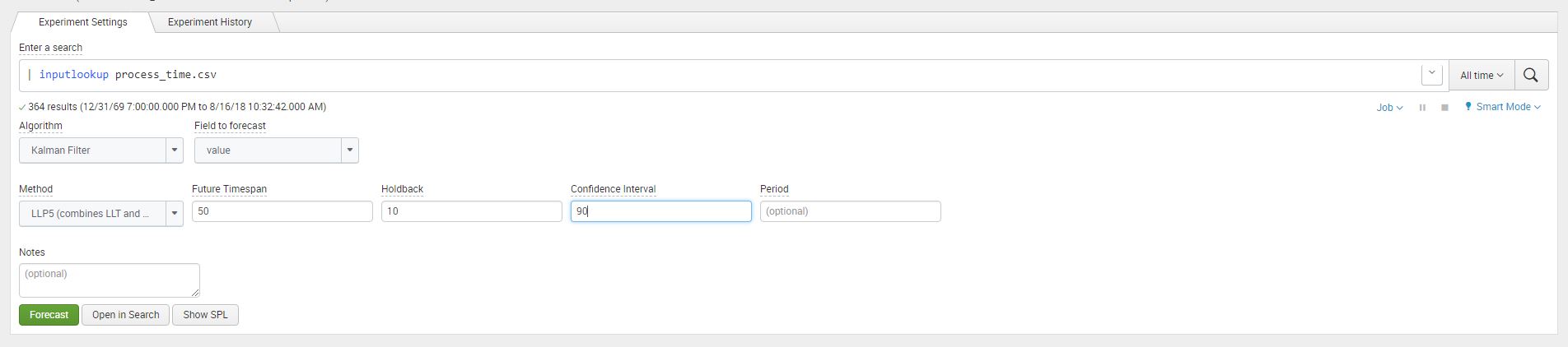
Once the argument values have been added click on ‘Forecast’ to display the visualization
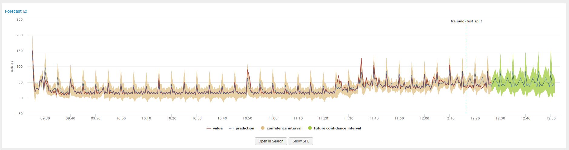
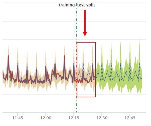
From the displayed line chart visual we can compare the accuracy of the test on the events that were retracted using the ‘holdback’ argument. Behind the dotted line is the data the algorithm used to learn and after the dotted line is the forecast for the next 50 events. The brown shaded area represents the test data after the dotted line.
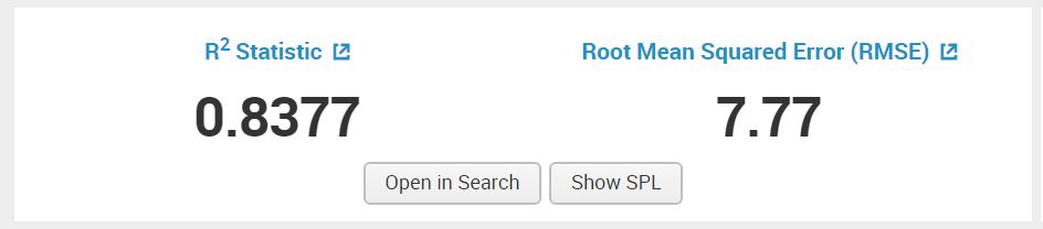
Another measure of accuracy is the R-Squared statistic in the below image, without going in depth about it, the closer it is to 1 the better the fit of the forecasted algorithm.
This method of forecasting is rather simple and less intensive on the computing side, allowing you to use it real-time in your Splunk queries. It is well documented in Splunk documents and through scholarly articles we can find resources explaining the mathematics on of this model. There are limitations listed in the Summary section below.
Summarising Kalman Filter in Splunk
Let’s summarise Kalman Filter usage in Splunk:
- You can execute the predict command in your SPL without excessive pre-formatting or complicated data manipulation
- We can use it to smooth out the time series for formatting
There are some limitations with this method for time series
- You can not rely on multiple seasonality in your data to be picked up accurately
- Kalman Filter can only be used for linear data sets. Decomposition or breaking of the non-linear components to linear data points can
- Some filters that are performed can cause loss of important information due to aggressive smoothing of the time series data
This concludes the first part of part of this blog. Part II of this blog will walk-though using ARIMA (AutoRegressive Integrated Moving Average) and determining the fit using Splunk’s Machine Learning Toolkit Interface.
Looking to expedite your success with Splunk? Click here to view our Splunk service offerings.
© Discovered Intelligence Inc., 2018. Unauthorised use and/or duplication of this material without express and written permission from this site’s owner is strictly prohibited. Excerpts and links may be used, provided that full and clear credit is given to Discovered Intelligence, with appropriate and specific direction (i.e. a linked URL) to this original content.

