Interesting Splunk MLTK Features for Machine Learning (ML) Development
The Splunk Machine Learning Toolkit is packed with machine learning algorithms, new visualizations, web assistant and much more. This blog sheds light on some features and commands in Splunk Machine Learning Toolkit (MLTK) or Core Splunk Enterprise that are lesser known and will assist you in various steps of your model creation or development. With each new release of the Splunk or Splunk MLTK a catalog of new commands are available. I attempt to highlight commands that have helped in some data science or analytical use-cases in this blog.
One of my favourite features in Splunk MLTK is the ‘Score’ command. It was released with MLTK version 4.0.0 and is packed with statistics such as AUC (Area Under the Curve) for classification models for model validation and ANOVA (Analysis of Variance) for linear regression models. This was a much awaited upgrade in Splunk MLTK when it was released. It provided metrics that are commonly used in the Data Science world for model verification and performance.
Before we begin – Let’s onboard some data in Splunk
I downloaded this dataset about predicting used-car prices based on several factors km_driven, field_type, seller_type etc from kaggle. Click here to download the car_dataset.csv file to follow this blog.
I added the csv file to my $SPLUNK_HOME/etc/apps/Splunk_MLTK/lookups/ directory. After onboarding the csv file use the ‘| inputlookup car_data.csv’ command to view the data.

Now that we have loaded some data lets go over the first useful command. It’s an eval function that can help create dummy variables for our categorical fields. It splits each field into separate fields based on the unique number of categorical values available in that column.
1 – Splunk: Creating dummy variables using Eval Command
Using the data loaded earlier, we can use eval to create dummy variables for the ‘Seller_Type’,’Transmission’,’Fuel_Type’ columns.
| inputlookup car_data.csv | eval dummy_{Seller_Type} = 1, dummy_{Transmission} = 1,dummy_{Fuel_Type} = 1
| fillnull value=0
The output of the SPL command is below. The dummy fields start with the addition of dummy* fields.
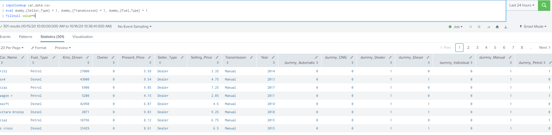
Dummy variables have a duel purpose, they can translate categorical or non-numeric columns into numeric by creating a cell
2 – MLTK: Score Anova Command for Ordinary Linear Regression Models
Also known as Analysis of Variance, it is a process through which the mean of two sample groups can be compared. It supplements hypothesis testing and general analysis of different populations. The following academic paper explains the importance of ANOVA extremely well. This can compliment your OLR (Ordinary Linear Regression) models for hypothesis testing as well as determine significance of each independent variable in your regression model.
The Anova command in Splunk contains configurable parameters such as adjusting the hetroskedastivity, or running a ‘f’ or ‘chi_squared’ test. We can even change the output table to view either the anova, model accuracy or independent coefficients tables. For a full list of configuration parameters, please look at Splunk MLTK document here. A point of clarification here is that the ‘|score anova command’ contains 3 different outputs, one which is the actual anova table, the second is a model accuracy table and the third is a table of coefficients.
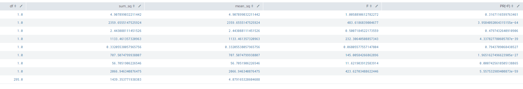
Anova Table
In the previous section we were able to create dummy variables for the categorical fields. Using the same dataset I can run the below command to output an anova table.
| inputlookup car_data.csv
| eval dummy_{Seller_Type} = 1, dummy_{Transmission} = 1, dummy_{Fuel_Type} = 1
| fillnull value=0
| score anova formula="Selling_Price ~ dummy_CNG + dummy_Diesel + dummy_Petrol + dummy_Dealer + dummy_Individual + dummy_Manual + dummy_Automatic + Present_Price" output=anova
Model Accuracy
The anova table is useful when analysis the regression model and to the untrained eye it just shows a lot of numbers, but lets change the output to model accuracy to determine how got the fit is of my model. I used the below SPL query:
| inputlookup car_data.csv
| eval dummy_{Seller_Type} = 1, dummy_{Transmission} = 1, dummy_{Fuel_Type} = 1
| fillnull value=0
| score anova formula="Selling_Price ~ dummy_CNG + dummy_Diesel + dummy_Petrol + dummy_Dealer + dummy_Individual + dummy_Manual + dummy_Automatic + Present_Price" output=model_accuracy

The model accuracy output will tell me the R_squared, Adjusted R_squared, AUC (covered below), F-Statistic and much more to determine the fit of my regression model. From the output of my result we can see that the Adjusted R_squared is 0.811 which means that I can explain about 81% of the variance of my selling price from the fields in the model.
Coefficients Table
The last output available with score anova is a table of efficient. We can view this table by changing the output to ‘coefficients’.
| inputlookup car_data.csv
| eval dummy_{Seller_Type} = 1, dummy_{Transmission} = 1, dummy_{Fuel_Type} = 1
| fillnull value=0
| score anova formula="Selling_Price ~ dummy_CNG + dummy_Diesel + dummy_Petrol + dummy_Dealer + dummy_Individual + dummy_Manual + dummy_Automatic + Present_Price" output=coefficients
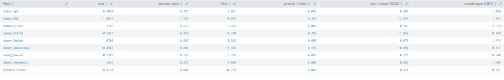
This output gives us the coeffecient of each variable, standard error, p-value and the t-stat associated with each of them. Without going into too much depth, you can also view the coefficients of each variable by running the ‘|summary’ command against your saved OLS model. However, this method will not give you the associated p-value and t-stats which each of the fields.
The output of the coefficients table is important to figure out if we should add or remove a field from our linear regression model. Generally speaking if the p-value is larger than 0.05 or 0.1 we would drop that field when we create the final model. A higher p-value than 0.05 or 0.1 shows less significance of that field in the model. Of course the decision to add or remove a field depends on the use-case the model developer has in mind.
3 – MLTK: T-tests
The t-tests are a very popular approach to determine if there are differences between two groups and if the differences are significant. Here are the 3 types of t-tests we can do with Splunk MLTK 5.2:
- One sample t-tests: This is used in to compare a sample mean against a population mean.
- Unpaired t-test: This test if two independent samples have a significant difference or not. This test is used when two samples consist of separate group of subjects
- Paired t-test: This test if two independent samples have a significant difference or not. This test is used when two samples are related
One sample t-tests:
From the dataset that we onboarded lets create a sample group to build and run each of the t-tests. I used the sample command to split my data in a 2:1 ratio where 1 will represent a sample of the cars data.
| inputlookup car_data.csv
| eval dummy_{Seller_Type} = 1, dummy_{Transmission} = 1, dummy_{Fuel_Type} = 1
| fillnull value=0 | sample seed=2607 partitions=3
| eval partition_number=if(partition_number>0,1,0) comment("splitting the data into 1/3rd sample and 2/3 population")
I will use partition 0 as my sample and I will test that against the mean of partition 1. In modeling terms we can consider partition 1 as a population (although not an ideal one). Using stats I was able to find the mean(average) of the Selling_Price field in partition 1. It came out to be 4.77. Now lets run a one sample t-test. Using the below SPL:
| inputlookup car_data.csv
| eval dummy_{Seller_Type} = 1, dummy_{Transmission} = 1, dummy_{Fuel_Type} = 1
| fillnull value=0
| sample seed=2607 partitions=3 | eval partition_number=if(partition_number>0,1,0)
| search partition_number=0
| score ttest_1samp Selling_Price popmean=4.77 alpha=0.1
This would show us the below table:

Assumption for the one-sided t-test: When we run the a one-sided t-test our null hypothesis will be that there is no difference between the mean of partition 0 and partition 1. This can be a complicated concept to grasp at first. From the resulting table, our t-statistic is -0.647 and our p-value is 0.518. We set our alpha in the SPL to be 0.1. We can see that the p-value of 0.518 is larger than the alpha we set of 0.1. As a result we can validate that there is no substantial difference between the mean of partition 0 and partition 1.
Unpaired t-test
The second type of t-test we can run is the Unpaired t-test. We use this to compare two different sets of values to determine if there a significant difference between the independent set of values. Lets seen how we can use the unpaired t-test.
We first have to create two different sets of values from our car_data.csv file. Using the search below I can create two different columns of Selling_Price using partition 0 and partition 1.
| inputlookup car_data.csv
| eval dummy_{Seller_Type} = 1, dummy_{Transmission} = 1, dummy_{Fuel_Type} = 1
| fillnull value=0
| sample seed=2607 partitions=3| search partition_number=0 | fields Selling_Price | rename Selling_Price as Selling_Price_0
| appendcols [| inputlookup car_data.csv | eval dummy_{Seller_Type} = 1, dummy_{Transmission} = 1, dummy_{Fuel_Type} = 1
| fillnull value=0 | sample seed=2607 partitions=3
| search partition_number=1 | fields Selling_Price
| rename Selling_Price as Selling_Price_1 ]
The result of the SPL will show two columns Selling_Price_0 and Selling_Price_1. We can now run the t-test by appending the below SPL to our search. I picked an alpha of 0.1
| score ttest_ind Selling_Price_1 against Selling_Price_0 alpha=0.1

Similar to the one-sided t-test given our extremely large p-value and alpha of 0.1 we can definitely reject our null-hypothesis when we run this unpaired t-test. Our null hypothesis in this case was that the Selling Price of Partition 0 and Selling Price of Partition 1 have different means. The Splunk output describes why the null-hypothesis was rejected in the ‘Test Decision’ column.
Commands in Classification Models AUC Score
Classification Models generally try and predict a discrete set of outcomes from your data. For example, predicting if a laptop is infected. Another example is if if a user will login or not. The two features I will cover today are ROC-AUC and the Correlation Matrix Command. Similar to Accuracy of a Classification Model, the ROC-AUC is another measure of determining the fit of your model on your test data. The Confusion Matrix feature was launched many MLTK versions ago. In my last blog about predicted Spam or not Spam I used SPL to create and generate a confusion matrix (how time flies).
ROC-AUC
Lets start with the ROC-AUC feature (Receiver Operating Characteristic – Area Under the Curve), it’s a performance measure of your classification model. A blog in TowardsData explains ROC and AUC brilliantly with its formulation. The fundamental analogy is that the higher the AUC score the better the model is, however the any score would need further context or comparison to determine how effective it is.
The AUC score can only be executed in your classification Model as shown below:
| inputlookup car_data.csv
| eval dummy_{Seller_Type} = 1, dummy_{Transmission} = 1, dummy_{Fuel_Type} = 1 | fillnull value=0| sample seed=2607 partitions=3 | search partition_number>0
| fit LogisticRegression "Seller_Type" from "Selling_Price" "dummy_Automatic" "Year" "dummy_Manual" "dummy_CNG" "dummy_Diesel" "dummy_Petrol" probabilities=True into "example_seller_dealer"
| score roc_auc_score Seller_Type against "probability(Seller_Type=Dealer)" pos_label='Dealer'

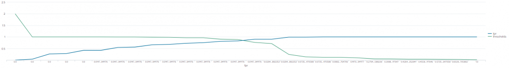
In the above example, the AUC Score is 0.989. Similar to the above SPL, we can plot the ROC-AUC Curve using the below command:
| inputlookup car_data.csv
| eval dummy_{Seller_Type} = 1, dummy_{Transmission} = 1, dummy_{Fuel_Type} = 1 | fillnull value=0 | sample seed=2607 partitions=3 | search partition_number>0
| fit LogisticRegression "Seller_Type" from "Selling_Price" "dummy_Automatic" "Year" "dummy_Manual" "dummy_CNG" "dummy_Diesel" "dummy_Petrol" probabilities=True into "example_seller_dealer"
| score roc_curve Seller_Type against "probability(Seller_Type=Dealer)" pos_label='Dealer'

Note that for both the above ROC curve and score examples, I’m running the score on the train dataset. In a production environment you would run that on your test dataset to improve your overall model.
Confusion Matrix
Confusion matrix is used to understand the performance of the data. However its calculation and terminology can be ‘confusing’. At it’s core it shows a number of values that areoriginally ‘Dealer’ and the model predicted correctly as ‘Dealer’ (true positive) and incorrectly as the ‘Individual’ (False Positive). The confusion matrix can be use to calculate the payoff on top of determining the correct predictions for your categorical model.
| inputlookup car_data.csv
| eval dummy_{Seller_Type} = 1, dummy_{Transmission} = 1, dummy_{Fuel_Type} = 1 | fillnull value=0 | sample seed=2607 partitions=3 | search partition_number>0
| fit LogisticRegression "Seller_Type" from "Selling_Price" "dummy_Automatic" "Year" "dummy_Manual" "dummy_CNG" "dummy_Diesel" "dummy_Petrol" probabilities=True into "example_seller_dealer"
| score confusion_matrix Seller_Type against "predicted(Seller_Type)"

Other ‘Honourable Mention’ Splunk Commands
AutoRegress
Autoregress in Machine Learning allows comparison between previous observations with your present observation for forecasting and additionally in calculating moving averages. In Splunk on top of its defined benefit it has many other useful features. Here are some use-cases that I’ve come across where I’ve used the autoregress command:
- Determining order of execution for playbooks/scripts
- Comparing previous and/or next value in a field for statistical comparison
- Validate login order for accounts of interest
The autoregress command is used to compare not just the previous value but any value at an Xth position. The SPL shown below demonstrations how you can use the autoregress command normally and if you want to compare a value with the 3rd one before it.
| inputlookup car_data.csv | streamstats count | eval Seller_Type=count+"-"+Seller_Type
| autoregress Seller_Type as previous_Seller_Type
| fields count *Seller_Type
| autoregress Seller_Type as previous_3rd_Seller_Type p=3

Correlation Matrix
The Correlation Matrix command can be used as a custom command and is well document in the Splunk MLTK documents. It outputs a matrix that shows the correlation coefficient of each of your selected fields with each other. The Splunk document contains the method to add the correlation matrix command to your SPL library here. An output of the correlation command should look like this:
| inputlookup firewall_traffic.csv| fields bytes packet | fit CorrelationMatrix method=kendall *

One of the best use of the correlation matrix is in preliminary analysis and in understanding correlation between fields in your data . If two fields are highly correlation the correlation matrix will show that, removing one of the correlation columns may improve the fit of your model.
The list of features in Splunk MLTK gets bigger and better with each new release of the application. If you would like us to expand on any existing or new feature in MLTK, feel free to reach out to us!
© Discovered Intelligence Inc., 2020. Unauthorised use and/or duplication of this material without express and written permission from this site’s owner is strictly prohibited. Excerpts and links may be used, provided that full and clear credit is given to Discovered Intelligence, with appropriate and specific direction (i.e. a linked URL) to this original content.


