
Predict Spam Using Machine Learning Classification
In this blog we will use a classification approach for predicting Spam messages. A classification approach categorizes your observations/events in discrete groups which explain the relationship between explanatory and dependent variables which are your field(s) to predict. Some examples of where you can apply classification in business projects are: categorizing claims to identify fraudulent behaviour, predicting best retail location for new stores, pattern recognition and predicting spam messages via email or text.
The aim of this blog post is to demonstrate a classification use case with the Splunk Machine Learning Toolkit. Manipulating and predicting any data involves understanding the raw data and scope of what you want to predict. In this blog, we want to predict spam messages. Before we can predict spam we need to understand what attributes/categories are there that define each message. For example: one category labelled ‘B’, can be presence of a special character such as {$,%,!,@} and so on. A message will be categorized into ‘B’ if it fits the criteria. Lets say that historically spam messages are defined by category ‘B’, when we analyze a new message and it contains a special character, there is a higher probability that it will classify as spam. The algorithm we work with in this blog works with this concept of probabilities to determine if a message is classified as spam or non-spam.
A blog on machine learning by Jason Brownlee outlines some of these steps, summarizing it from the site [Jason Brownlee, 2018]:
- Peek at your raw data: Observing the raw data gives insight into how the data is structured, providing insights for pre-processing
- Dimensions of your data: Too many fields or even lack of fields will impact the accuracy of the algorithm
- Data Type for Each field: Fields that are strings may need to be converted to values to represent categories
- Correlation between fields: Correlation between fields bring in the same information and would impact your logistic regression model by adding data bias
Understanding the Data Set
A sample dataset was constructed with events artificially categorized to understand how Machine Learning can be used for statistical analysis and prediction. Click email_dataset.csv to download the dataset.
Email_dataset.csv contains sample email subjects in column ‘A’ and the remaining columns headers contain the categories the email subject fits into. Some examples of the categories are listed below, the first column contains only raw subject header text:
email_subject_text: (first column) Displays sample email subjects
spam: This is the observed binary variable indicating if email is spam or not. Binary variable is such that it can only be one of two values {0,1}.
subject_contain_spam_keywords: Binary variable indicating if the email subject contains spam keywords
subject_contains_special_characters: Binary variable indicating if the email subject contains special characters
mail_client: Lists the email clients the sender used. To use this field with logistic regression we assigned each mail client a unique number e.g Outlook 2013: 1; Thunderbird:2 and so on. This pre-processing step allows the data to be used in the algorithm.
In our data we have a column header ‘spam’ which categorizes the data into ‘spam’ (indicated by 1) or ‘not spam’ (indicated by 0). It is important to have this column so that the algorithm can learn which categories (such as spam words, special characters etc) contributed to classifying an email subject as spam. Two rows from the dataset are posted below for reference (The Mail Client field in this example shows the proper client name for reference):
Email Subject Text |
Spam |
Does Subject Contain Spam keyboards |
Subject Contains Special Characters |
Mail Client |
| Free Watches!! | 1 | 1 | 1 | Outlook 2013 |
| Links to Cloud Document | 0 | 0 | 0 | Thunderbird |
Prerequisites of the Model
Before processing the data, here are two key mathematical assumptions for the models and data [Dr James Lani]:
- Little or No multicollinearity: Multicollinearity is caused due to inclusion of categories that are derived from other categories. This could make it difficult for the algorithm to asses the impact of each of the independent category. For example if we have a category ‘subject_contains_special_characters’ and ‘subject_contains_dollar_sign_$’ these two categories are defined as multicollinear because a dollar sign will always fall in a special character category
- Homoscedasticity: Each field/attribute has a limited variance, which means that there are finite values each field can have. This can affect the fit of the regression algorithm impacting the prediction. A limited or smaller number of unique values each category allows the algorithm to calculate the probability easier
Further assumptions and their descriptions can be read from Statistic Solutions blog in the references. For simplicity we are walking through the tools of using this model in Splunk rather focusing on the mathematical theory.
Our Questions
We will be using logistic regression for our predictive analysis to determine if an email is spam or not. It will help answer our questions on:
- Is the model accurate in classifying spam messages?
- Do the categories such as: mail_client, priority, internal_gl, subject_contains_special_characters etc. have any influence on the email being spam?
Logistic Regression Algorithm
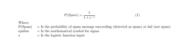
Despite its name ‘Logistic Regression’ is an algorithm for classification. In this algorithm, the probabilities detailing the outcome of our field of interest are modeled using a logistic function which is the basic equation in logistic regression. The outcome of logistic regression is a simple binary result ‘1’ or ‘0’ signifying if an email is a spam or not.
Without delving too deep into the mathematics of the algorithm, the logistic regression is built upon a logistic function which is shown in the screenshot below. The logistic function gives a value between 0 and 1 for the input variables, which enables the algorithm to decide if its spam or not.
Training the Logistic Regression Algorithm Using SPL
Once the dataset has been uploaded, we can use the following ML-SPL to partition the data into 4 groups, allowing the equation to learn from 3 out of the 4 groups. We will then use the 4th partition to test the accuracy of our results when we make our prediction. Please ensure that the Splunk queries are executed from the MLTK Search page to avoid any permission issues on using custom commands that are imported with the MLTK app.
| inputlookup email_dataset.csv
 | sample partitions=4 seed=123456
 | search partition_number<3
 | fields - "priority"
 | fit LogisticRegression fit_intercept=true "spam?" from "characters_in_subject" "does_the_subject_contain_spam_keywords?" "email_is_reply_chain?" "header_contains_an_image?" "internal_gl?" "language" "mail_client" "plain_text_email_type?" "return_path_different_then_sender?" "subject_contains_emojis?" "subject_contains_exclamation_marks?" "subject_contains_numeric_values" "subject_contains_periods?" "subject_contains_special_characters?" into "LogRegres_Spam_Model"
Breaking down the Splunk query from top-down:
- Line 1: Inputlookup command displays the email_dataset csv file we uploaded
- Line 2: The Sample command splits the data into 4 partitions. The partitions start from 0 to 3, with 3 as the 4th partition
- Line 3: Narrows down the data to the show partition 0,1,2 for the algorithm to learn/train from by adding condition ‘search partition_number<3’
- Line 4: Removes the ‘priority’ field from the table that as we are not using that in the logistic regression algorithm
- Line 5: Lastly, we are using the ‘fit command to apply the LogisticRegression algorithm to predict the field ‘spam?’ based on the explanatory variables “characters_in_subject”, “does_the_subject_contain_spam_keywords?” and so on…
- Line 5: The ‘into’ command saves the model as ‘LogRegres_Spam_Model’. If a model is not provided it will save the model as ‘default_model_name‘
Using the Trained Model to Predict Unseen Data
As a general rule, we should always reserve a percentage of data the model has not learned to test the accuracy of our result. The next step is to ‘apply’ the model to partition_number 3, which contains the data the model has not seen. We will use the results to validate the accuracy of our model.
| inputlookup email_dataset.csv
 | sample partitions=4 seed=123456
 | search partition_number=3
 | apply "LogRegres_Spam_Model" as "Spam_prediction"
We will call this search “ base prediction search” for referencing in the blog in the next few sections. The data of the base prediction search would show in tabular format as shown below:
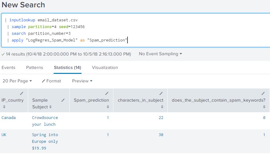
From our Splunk Query we can see that an alias ‘Spam_prediction’ was used for the ‘predicted(Spam?)’ field. From the table we can verify that Spam_prediction and ‘Spam?’ are both fields present in the search.
View the Results as a Table
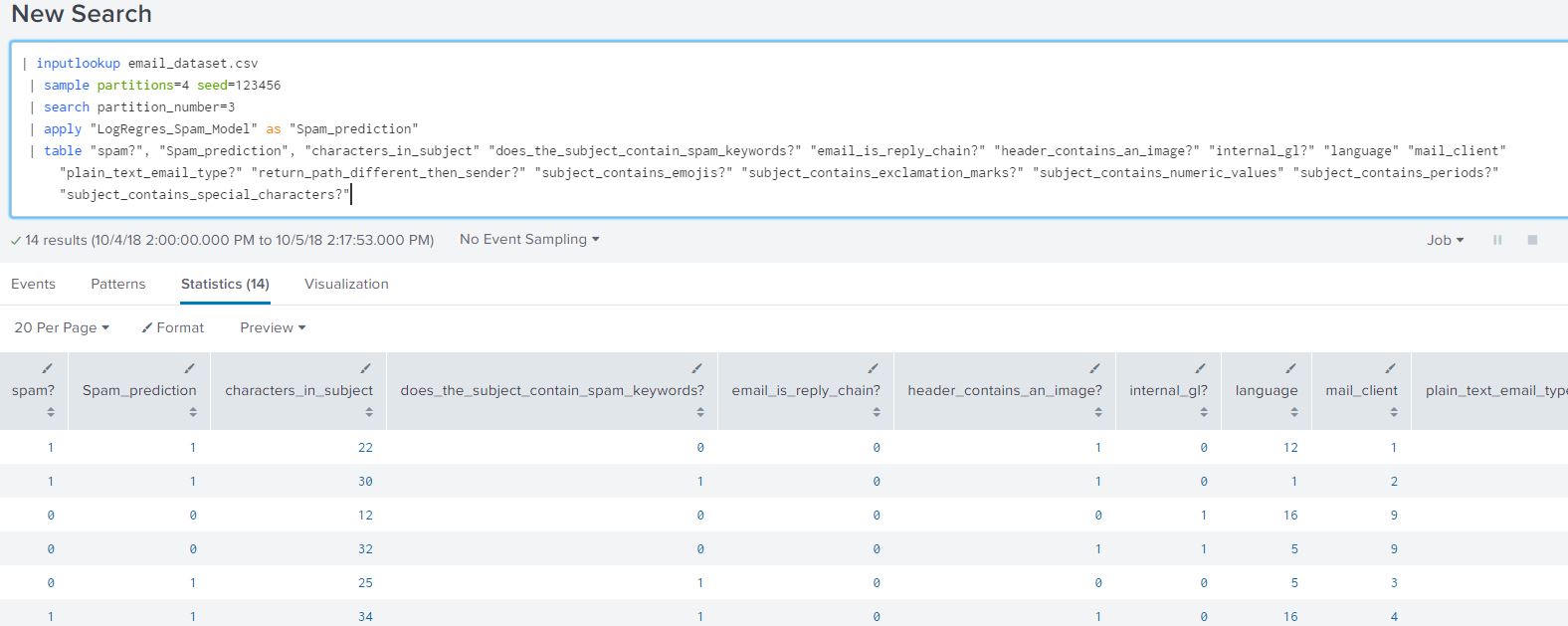
Append the below query to the base prediction search to view the raw results of the model:
| table "spam?", "Spam_prediction", "characters_in_subject" "does_the_subject_contain_spam_keywords?" "email_is_reply_chain?" "header_contains_an_image?" "internal_gl?" "language" "mail_client" "plain_text_email_type?" "return_path_different_then_sender?" "subject_contains_emojis?" "subject_contains_exclamation_marks?" "subject_contains_numeric_values" "subject_contains_periods?" "subject_contains_special_characters?"
Viewing the results as raw data helps us view what the expected outcome of the algorithm looks like. It would give us a the value ‘1’ for any email that is likely to be spam or ‘0’ otherwise.
Analyzing Model Statistics for Understanding The Result
Model Error Statistics
To view the model error statistics we append a pre-defined macro from the Machine Learning Toolkit app to the base prediction search to get the model statistics.
| `classificationstatistics(“spam?”, “Spam_prediction”)`
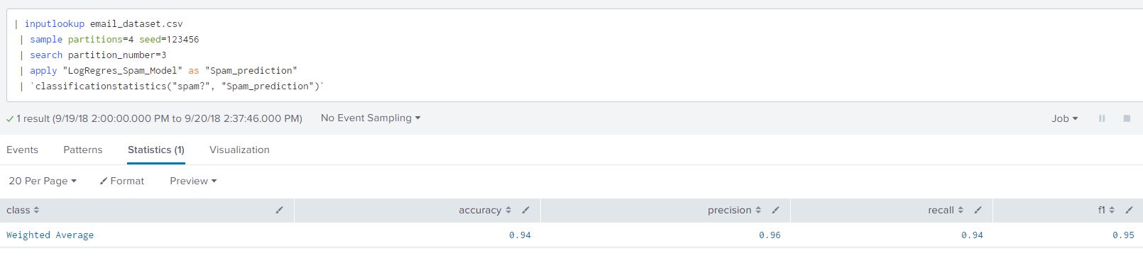
This gives us the accuracy, precision, recall and f1 of the algorithm. The closer the values are to 1 the better the fit of the model for each of the headers. Each of the table headers in the classification statistics mentions an method of estimating accuracy of our classification. These measurements can be calculated from the confusion matrix. We will describe the the method of calculating accuracy in the results section and for simplicity will not delve into the remaining measurements. We can read Jason Brownlee’s article in the links provided on classification accuracy and other methods of measuring predictable capability of the model.
Confusion Matrix
A confusion matrix is a popular analytical matrix that lays out the performance of this algorithm on ‘unseen’ (or paritition_number=3 in our dataset), it lists results that it has correctly predicted. Append the below query to the base prediction search to view the confusion matrix.
| `confusionmatrix("spam?", "Spam_prediction")`
The result will be a table as shown below:
| Actual Data | Predicted 0 | Predicted 1 |
| 0 (Not Spam) | 4 | 1 |
| 1 (Spam) | 0 | 9 |
In our partition_number 3 there were 14 data points which the classification model had not seen. This table compares the values of what the model predicted and what the actual result is from the 14 raw data points. Reading this numeric table can get complicated as it represents more then just numbers, its also a measure of accuracy of our classification model.
Before we interpret the table, we use SPL to calculate the column and rows totals. I added the below search after the confusion matrix command to sum the column and rows. Calculating the sum is important to identify the false and true positives predictions of the model.
| `confusionmatrix("spam?", "Spam_prediction")`
| addtotals labelfield="Predicted actual" | rename Total as "row_total"
| addcoltotals label="col_total" labelfield="Predicted actual"
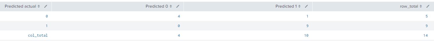
We have added some mathematical terms to each of the cells from the confusion matrix in the table below.
| Predicted actual | Predicted 0 | Predicted 1 | row_total |
| 0 (Not Spam) | 4 (True Negative) | 1 (False Positive) | 5 |
| 1 (Spam) | 0 (False Negative) | 9 (True Positive) | 9 |
| col_total | 4 | 10 | 14 (Total Data Points) |
Explaining the terminology from the table will help explain the confusion matrix further:
- True Positive: When the email is actual spam, how often does the model predict spam? From our data set we can see that predicts spam correctly with an accuracy of 100% (9 out of 9 times it has predicted spam corrected, this may not be the case in most applications)
- False Positive: When the data is not spam how often does it predict it as spam? From the table we can calculate it to be 20% (1 out of 5 times)
- False Negative: When the data is spam but the model predicts it as not spam? From the table we can calculate it to be 0% (0 out of 9 times)
- True Negative: When the data is not spam but the model predicts it correct as not spam. From the data we can calculate it as 80%, since 4 out of 5 times the ‘not spam’ data points were predicted correctly
These terms make up the predictive capability of the model and help in judging the accuracy of classification when you have large datasets rather than analyze how fast or scalable the model is. The confusion matrix is also the backbone for computing other statistical relevant terms such as precision, false positive rate, true positive rate. From confusion matrix we will jump onto the next available statistic from the MLTK.
Field Coefficients
The coefficients of each field tell us about the relationship between each field and the input field (“Spam?”). They estimate the amount of increase in the predicted ‘log odds’ of an email recognized positively as spam (or Spam =1). For simplicity and relevancy, we will not be jumping into the concept of log odds. You can read further about log it from the reference links.
| summary LogRegres_Spam_Model
Using the above summary command, we can see the coefficients of the fields with respect to the input field (“Spam?”).
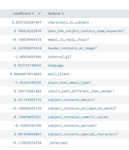
A positive coefficient 0.029 for the field ‘characters_in_subject’ tells us that for one unit increase in the characters we would expect an increase the likelihood for the spam.
A negative coefficient -2.088 for the field ‘internal_gl’ tell us that for one unit increase in ‘internal gl’ we will expect a decrease in the likelihood of spam.
Using this method we can make say with a certain degree of confidence how each of the input fields in our data sets impact our prediction. A use case of this is the identification of inputs fields that are major contributors to the event/data classified as spam.
Results
From the previous section we understand that fields with higher positive co-efficient from the previous section have a higher change of contributing to an email categorized as spam. Based off the confusion matrix we can calculate by using a simple formula (True Positive + True Negative)/Total Data Points = (9+4)/14 = ~0.93 or 93%. This tells us that in general the model is correct 93%.
This statistic is based off the data from the sample data dataset, it would vary in each machine learning application and use case of the data being investigated.
Summarizing the Steps
- Upload Dataset
- Select data partition size (e.g use 75% for learning and 25% for testing)
- Use algorithm to training data and save model
- Apply saved model to test data
- Analyze model results
- Schedule Alert and/or other action(s)
From this blog we hope to have provided you the tools to detect and analyze patterns in your own environment. There are pre-requisites required such as extracting, cleaning and transforming the data for machine learning. The processing stage of data for classification can be complex especially if no existing mechanism exists to categorize data before we start processing it.
If you have any questions on how to implement this in your Splunk, please feel free to reach out to us.
References and Links
Jason Brownlee, 2016, Understand Your Machine Learning Data Descriptive Statistics Python
https://machinelearningmastery.com/understand-machine-learning-data-descriptive-statistics-python/
Dr. James Lani, 2018, Assumptions of Logistic Regression
https://www.statisticssolutions.com/assumptions-of-logistic-regression/
Institute for Digital Research and Education, UCLA, 2018, Logistic Regression Analysis
https://stats.idre.ucla.edu/stata/output/logistic-regression-analysis/
Splunk Documentation on MLTK Search Commands, 2018, Custom Search Commands
https://machinelearningmastery.com/classification-accuracy-is-not-enough-more-performance-measures-you-can-use/
Jason Brownlee, 2014, Classification Accuracy is Not Enough
https://blog.exsilio.com/all/accuracy-precision-recall-f1-score-interpretation-of-performance-measures/
7 Use Cases For Data Science And Predictive Analytics
https://towardsdatascience.com/7-use-cases-for-data-science-and-predictive-analytics-e3616e9331f9
© Discovered Intelligence Inc., 2018. Unauthorised use and/or duplication of this material without express and written permission from this site’s owner is strictly prohibited. Excerpts and links may be used, provided that full and clear credit is given to Discovered Intelligence, with appropriate and specific direction (i.e. a linked URL) to this original content.


