Are you having trouble managing thousands and thousands of Splunk forwarders? Until now, many organizations have typically used numerous deployment servers in a scaling configuration, to manage a massive number of forwarders.
However, to make life easier, Splunk has introduced a new feature called ‘Deployment Server Clustering’, which was introduced with Splunk version 9.2.
https://discoveredintelligence.com/wp-content/uploads/2024/04/deployment_server_clustering.jpg6311000Discovered Intelligencehttps://discoveredintelligence.com/wp-content/uploads/2013/12/DI-Logo1-300x137.pngDiscovered Intelligence2024-04-23 14:01:572025-12-17 16:27:26Deployment Server Clustering – An Easier Way to Manage Splunk Forwarders
In today’s data-driven world, mastering the Splunk Search Processing Language (SPL) is essential for effective data analysis. However, for beginners, SPL can seem like a daunting language to learn. Enter the Splunk AI Assistant – a revolutionary tool designed to make SPL accessible to users of all levels of expertise.
https://discoveredintelligence.com/wp-content/uploads/2024/04/splunk_ai_assistant.jpg8141200Discovered Intelligencehttps://discoveredintelligence.com/wp-content/uploads/2013/12/DI-Logo1-300x137.pngDiscovered Intelligence2024-04-09 13:06:202025-12-17 16:28:33Simplifying SPL: A Beginner’s Guide to the Splunk AI Assistant
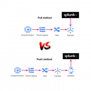
In this blog we will talk about the processes and the options we have to collect the GCP events and we will see how to collect those in Splunk. In addition, we will even add integration with Cribl, as an optional step, in order to facilitate and optimize the process of information ingestion. After synthesizing all of this great information, you will have a great understanding of the available options to take, depending on the conditions of the project or team in which you work.
https://discoveredintelligence.com/wp-content/uploads/2023/08/gcp_splunk_spotlight.png400600Discovered Intelligencehttps://discoveredintelligence.com/wp-content/uploads/2013/12/DI-Logo1-300x137.pngDiscovered Intelligence2023-08-09 16:34:142023-08-29 01:04:31Building a Unified View: Integrating Google Cloud Platform Events with Splunk
Are you tired of hardcoding email addresses into your searches and alerts? Do you want a more dynamic way to send search results to individuals based on the data within your search results? Look no further than SendResults, a powerful Splunk command and alert action developed by Discovered Intelligence.
https://discoveredintelligence.com/wp-content/uploads/2023/08/sendresults_command.png400600Discovered Intelligencehttps://discoveredintelligence.com/wp-content/uploads/2013/12/DI-Logo1-300x137.pngDiscovered Intelligence2023-08-09 14:55:212025-12-17 16:28:41Discover the Power of SendResults: A Life-Changing Splunk Command and Alert Action
If you haven’t heard of ChatGPT yet, you likely have blocked notifications on social networks like Linkedin, Twitter or Reddit, as everyone is talking about the benefits (and concerns) of artificial intelligence. However, it’s ChatGPT who gets the lion’s share of the limelight in this story.
https://discoveredintelligence.com/wp-content/uploads/2023/05/chatgpt_help.png353685Carlos Moreno Buitragohttps://discoveredintelligence.com/wp-content/uploads/2013/12/DI-Logo1-300x137.pngCarlos Moreno Buitrago2023-05-31 23:53:072023-06-01 13:53:05ChatGPT and SPL: A Dynamic Duo for Learning Splunk’s Query Language
Organizations of all sizes are building / migrating / refactoring their software to be cloud-native. Applications are broken down into microservices and deployed as containers. Consequently there has been a seismic shift in the complexity of application components thanks to the intricate network of microservices calling each other. The traditional sense of “monitoring” them no longer makes sense, especially because containers are ephemeral in nature and are treated as cattle, instead of as pets.
https://discoveredintelligence.com/wp-content/uploads/2023/05/k8s_otel_collection.jpg440800Discovered Intelligencehttps://discoveredintelligence.com/wp-content/uploads/2013/12/DI-Logo1-300x137.pngDiscovered Intelligence2023-05-12 14:25:572025-12-17 16:29:39Wiring up the Splunk OpenTelemetry Collector for Kubernetes
Workload management is a powerful Splunk Enterprise feature for users to delegate CPU and memory resources to various Splunk workloads, based on their preferences. As Splunk continues to develop new attributes for the defining of rules, the number of Splunk users who are enabling workload management in their environment is gradually increasing.
The quote from Check Point Research above illustrates where the future trend of cybersecurity is headed and the challenges that organizations must face. However, anticipating and preparing the system defenses to evade and mitigate these attacks is not an easy task. From defining response and incident strategies to preparing work teams and configuring monitoring systems, it can all be a challenge.
Your core business is not to detect and mitigate security attacks, but is this essential to the achievement of your objectives? Have you ever wondered how you can simulate attacks and detections within a controlled environment to validate the configuration of your detection systems without spending part of your annual security budget? Read on and discover Splunk Attack Range.
What is Splunk Attack Range?
Splunk Attack Range is a tool developed by Splunk Threat Research Team (STRT) to simulate cyber attacks in a controlled environment for the purpose of improving an organization’s security posture. It allows security teams to test and validate their detection and response capabilities against a wide range of attack scenarios and techniques, such as phishing, malware infections, lateral movement, and data exfiltration.
Splunk Attack Range is designed to work with Splunk Enterprise Security, which is a security information and event management (SIEM) solution, and includes pre-built attack scenarios that are aligned with the MITRE ATT&CK framework, these ones can be customized to simulate the specific threats and vulnerabilities that are relevant to an organization’s environment.
Where can I get Attack Range?
The STRT and the Splunk community are maintaining the project in GitHub.
Is Splunk Attack Range Easy to Deploy?
Yes, it is really straightforward! You can deploy it locally (if you have a powerful machine), on Azure or on AWS. Internally, we use our AWS environment and with a few simple steps, in a matter of minutes, terraform and ansible automatically deploy a complete test lab to validate our customers’ security configurations and optimize the security posture with Splunk’s real-time monitoring. This process allows for a proactive approach to managing security postures with Splunk and saves a lot of time for your Blue Team.
…and now?
Have fun! By merging our Splunk expertise and using these kinds of automation tools, we have been able to speed up our internal testing processes, stay agile and secure with Splunk’s security posture management tool, and transfer this knowledge and configurations on to our customers’ cybersecurity teams.
We strongly encourage you to try this tool. Check out an overview of v1.0, v2.0 and v3.0 in the Splunk blog.
https://discoveredintelligence.com/wp-content/uploads/2023/03/splunk-attack-range-logo-e1678466676167.png693696Carlos Moreno Buitragohttps://discoveredintelligence.com/wp-content/uploads/2013/12/DI-Logo1-300x137.pngCarlos Moreno Buitrago2023-03-14 15:17:262023-03-14 15:17:29Save Time and Improve your Security Posture with Splunk Attack Range
Once you have embraced and grasped the power of Cribl Stream, “Reduce! Simplify!” will become your new mantra.
Here we list some of the best Cribl Stream resources available to get you started. Most of these resources are completely free! – money is not an obstacle when beginning your Cribl Stream journey, so keep reading and start learning today!
https://discoveredintelligence.com/wp-content/uploads/2023/02/getting_started_with_cribl.png582550Terry Mulliganhttps://discoveredintelligence.com/wp-content/uploads/2013/12/DI-Logo1-300x137.pngTerry Mulligan2023-02-23 15:20:382024-01-19 02:44:06Help Getting Started with Cribl Stream
Deploying apps to forwarders using the Deployment Server is a pretty commonplace use case and is well documented in Splunk Docs. However, it is possible to take this a step further and use it for distribution of apps to the staging directories of management components like cluster manager or a search head cluster deployer, from where apps can then be pushed out to clustered indexers or search heads.