Upgrading on-premise Linux Splunk Enterprise instances has historically been a complex and challenging task, but the new Upgrader App for Splunk (UA4S) app is designed to change that. In this review, we’ll take a closer look at how this app simplifies the upgrade process and makes this task accessible for anyone, even those without extensive technical expertise.
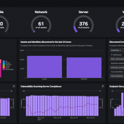
Splunk Asset and Risk Intelligence (ARI) enables your team to quickly perform complete and thorough asset investigations. An interactive and holistic approach provides security teams with much needed context about assets, including asset health, network activity and associations.
Have you ever wished you had a fresh ephemeral Splunk instance that you could quickly spin up, run some tests and then kill it, with maximum speed and minimum cloud costs?
Enter Hashi Terraform to the rescue. The industry-leading infrastructure-as-code tool makes the standup, setup and teardown of cloud compute nodes simple, speedy and repeatable so that an environment can be built, a complete set of tests can be run, results received and the test nodes destroyed in minutes rather than hours.
In this whitepaper, I show how I set up my computer and built the Search Head and Deployment server, as well as how I set up the many Splunk Universal Forwarders to satisfy the test plan.
Download Whitepaper
Get access to this exciting whitepaper now, by completing the form below.
https://discoveredintelligence.com/wp-content/uploads/2024/08/di_terraform_gcp_splunk_whitepaper.jpg6821000Darren Fullerhttps://discoveredintelligence.com/wp-content/uploads/2013/12/DI-Logo1-300x137.pngDarren Fuller2024-09-09 15:35:512024-10-04 13:49:48Setting Up a Splunk Testing Environment Using Terraform & GCP
Splunk Asset and Risk Intelligence (ARI) continuously discovers all assets on the network using a unique approach that creates a single source of truth from multiple sources of record, resulting in comprehensive and accurate asset visibility and reporting.
Splunk Asset and Risk Intelligence (ARI) is a powerful, premium application from Splunk which delivers proactive risk mitigation through continuous asset discovery and compliance monitoring.
If you are like me when I started with Cribl, you will have plenty of Splunk knowledge but little to no Cribl experience. I had yet to take the training, had no JavaScript experience, and only had a basic understanding of Cribl, but I didn’t let that stop me and just dove in. Then I immediately struggled because of my lack of knowledge and spent countless hours Googling and asking questions. This post will list the information I wish I had possessed then, and hopefully make your first Cribl experience easier than mine.
Cribl Quick Reference Guide
If I could only have one item on my wish list, it would be to be aware of the Cribl Quick Reference Guide. This guide details basic stream concepts, performance tips, and built-in and commonly used functions.
Creating that first ingestion, I experienced many “how do I do this” moments and searched for hours for the answers, such as “How do I create a filter expression?” Generally, filters are JavaScript expressions essential to event breakers, routes, and pipelines. I was lost unless the filter was as simple as 'field' == 'value.' I didn’t know how to configure a filter to evaluate “starts with,” “ends with,” or “contains.” This knowledge was available in the Cribl Quick Reference Guide in the “Useful JS methods” section, which documents the most popular string, number and text Javascript methods.
Common Javascript Operators
Operator
Description
&&
Logical and
||
Logical or
!
Logical not
==
Equal – both values are equal – can be different types.
===
Strict equal – both values are equal and of the same type.
!=
Returns true if the operands are not equal.
Strict not equal (!==)
Returns true if the operands are of the same type but not equal or are of different kinds.
Greater than (>)
Returns true if the left operand is greater than the right operand.
Greater than or equal (>=)
Returns true if the left operand is greater than or equal to the right operand.
Less than (<)
Returns true if the left operand is less than the right operand.
Less than or equal (<=)
Returns true if the left operand is less than or equal to the right operand.
Regex
Cribl uses a different flavour of Regex. Cribl uses ECMAScript, while Splunk uses PCRE2. These are similar, but there are differences. Before I understood this, I spent many hours frustrated that my Regex code would work in Regex101 but fail in my pipeline.
Strptime
It’s almost identical to the version that Splunk uses, but there are a few differences. Most of my problems were when dealing with milliseconds. Cribl uses %L, while Splunk uses %3Q or %3N. Consult D3JS.org for more details on the strptime formatters.
JSON.parse(_raw)
When the parser function in a pipeline does not parse your JSON event, it may be because the JSON event is a string and not an object. Use an eval function with the Name as _raw and the Value Expression set to JSON.parse(_raw), which will convert the JSON to an object. A side benefit of JSON.parse(_raw) is that it will shrink the event’s size, so I generally include it in all my JSON pipelines.
Internal Fields
All Cribl source events include internal fields, which start with a double underscore and contain information Cribl maintains about the event. Cribl does not include internal fields when routing an event to a destination. For this reason, internal fields are ideal for temporary fields since you do not have to exclude them from the serialization of _raw. To show internal fields, click the … (Advanced Settings) menu in the Capture window and toggle Show Internal Fields to “On” to see all fields.
Event Breaker Filters for REST Collector or Amazon S3
Frequently, expressions such as “sourcetype=='aws:cloudwatchlogs:vpcflow‘” are used in an Event breaker filter, but sourcetype cannot be used in an Event Breaker for a REST Collector or an Amazon S3 Source. This is because this sourcetype field is set using the input’s Fields/Metadata section, and the Event Breaker is processed before the Field/Metadata section.
For a REST collector, use “__collectible.collectorId=='<rest collector id>'” internal field in your field expression, which the REST collector creates on execution.
One of Cribl Stream’s most valuable functions is the ability to effortlessly drop fields that contain null values. Within the parser function, you can populate the “Fields Filter Expression” with expressions like value !== null.
Some example expressions are:
Expression
Meaning
value !== null
Drop any null field
value !== null || value==’N/A’
Drop any field that is null or contains ‘N/A’
Once I obtained these knowledge nuggets, my Cribl Stream was more efficient. Hopefully, my pain will be your gain when you start your Cribl Stream journey.
https://discoveredintelligence.com/wp-content/uploads/2024/06/things_i_wish_i_knew_cribl.png532800Terry Mulliganhttps://discoveredintelligence.com/wp-content/uploads/2013/12/DI-Logo1-300x137.pngTerry Mulligan2024-07-08 13:00:002024-07-08 17:05:59Cribl Stream: Things I wish I knew before diving in
At the recent Splunk .Conf in Las Vegas a couple of weeks ago, we were able to get a detailed demo of Splunk’s new and exciting Splunk Asset and Risk Intelligence (Splunk ARI) security solution. What a great solution and one that is much needed within their security solution portfolio. Splunk ARI falls into a category of products known as CAASM – Cyber Asset Attack Surface Management. In this post, we dive a little deeper into what CAASM is, why it is critical tool for your organization and how Splunk ARI can help.
https://discoveredintelligence.com/wp-content/uploads/2024/06/ari_homepage.png4651000Discovered Intelligencehttps://discoveredintelligence.com/wp-content/uploads/2013/12/DI-Logo1-300x137.pngDiscovered Intelligence2024-07-02 09:00:002024-07-17 14:09:26Splunk Asset and Risk Intelligence – a CAASM Solution for Splunk
Still winding down from the incredible experience at .conf24, where we delved into the latest market trends, we’ve uncovered several fascinating enhancements for the Splunk platform. These improvements not only elevate the performance and efficiency of Splunk but also offer exciting features that will be available in future releases. Join us as we explore four powerful upgrades that can be used in your Splunk environment.
https://discoveredintelligence.com/wp-content/uploads/2024/06/splunk_training_video.jpg613900Discovered Intelligencehttps://discoveredintelligence.com/wp-content/uploads/2013/12/DI-Logo1-300x137.pngDiscovered Intelligence2024-06-11 15:36:522024-06-26 15:53:53Learning Splunk with the new ‘Getting Started with Splunk’ Video Series
April marked the beginning of a new era for Cribl with the introduction of Cribl Lake, which brings Cribl’s suite of products full circle in the realm of data management. In this post we dive a bit deeper into some of the benefits and features of Cribl Lake.
https://discoveredintelligence.com/wp-content/uploads/2024/05/cribl-lake-1.png354553Discovered Intelligencehttps://discoveredintelligence.com/wp-content/uploads/2013/12/DI-Logo1-300x137.pngDiscovered Intelligence2024-06-06 16:21:352024-06-06 16:30:10Introducing the benefits and features of Cribl Lake