A Practical Example Using The Splunk Machine Learning Toolkit
In our previous blog we walked through steps on installing the Splunk Machine Learning Toolkit and showcased some of the analytical capabilities of the app. In this blog we will deep dive into an example dataset and use the ‘Predict Numeric Fields’ assistant to help us answer some questions about it.
The sample dataset used is from People’s dataset repository [Houghton] This multivariate sample dataset contains the following fields:
- Net Sales/$ 1,000
- Square Feet/ 1,000
- Inventory/$ 1,000
- Amt Spent on Advertising/$ 1,000
- Size of Sales District/1000 families
- No of Competitors in district
You can download a copy of the sample data here: greenfranchise.csv
What Questions do we want to ask?
We would like to understand the relationship between ‘Net Sales’ of Green Franchise and how it is impacted by the variables ‘Square Feet of Store’, ‘Inventory’, ‘Amount Spent on Advertising’, ‘Size of Sales District’ & ‘No of Competitors’. E.g Would an increase in ‘Inventory’ or ‘Amount Spent on Advertising’ increase or decrease ‘Net Sales’ for Greens?
The next few sections will walk you through uploading the data set and processing it in the Machine Learning Toolkit App.
Uploading the Sample Data Set
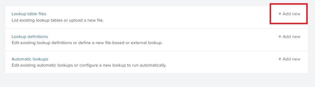
The CSV file was uploaded to Splunk from Settings -> Lookups -> Lookup table files (Add new). If you need more information on this step please consult the Splunk Docs here. Save the CSV file as greenfranchise.csv
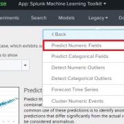
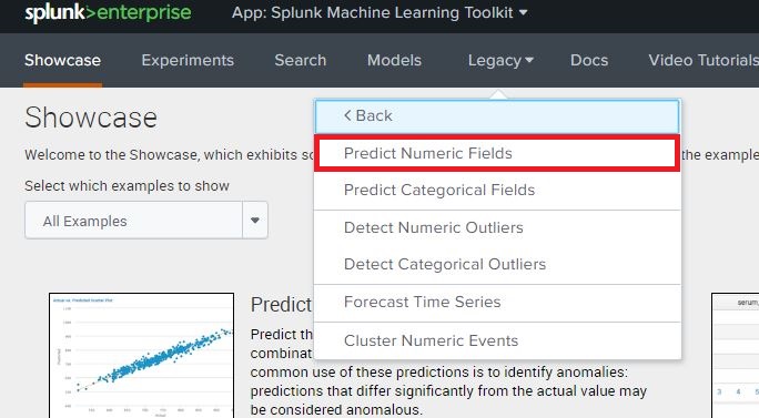
Once the file has been uploaded and saved as greenfranchise.csv, navigate to the Splunk Machine Learning Toolkit App, click on the ‘Legacy’ menu, Assistants and open the ‘Predict Numeric Fields’ Assistant. This screenshot and navigation may differ depending on which version of Splunk and the MLTK is installed. Assistants in version 3.2 can be found under the ‘Legacy’ tab.
App: Splunk Machine Learning Toolkit
Populate Model Fields
In the Create New Model tab, you can view the contents of the CSV file by running the below Splunk Query in the Search bar:
| inputlookup greenfranchise.csv
This will automatically populate the panels with the fields in the csv file. Below the “Preprocessing Steps” we can see a second panel to choose the type of algorithm to apply to this lookup.

Selecting the Algorithm
In the panel for selecting the algorithm, we can see the ‘Fields to predict’ and ‘Fields to use for predicting’ fields are automatically populated from the data. For this test we use the linear regression algorithm to forecast the ‘Net Sales’ of Green Franchises. Select “Net Sales” as the Field to predict, and in the Fields to use for predicting, select all of the remaining fields except for “Size of Sales District”.
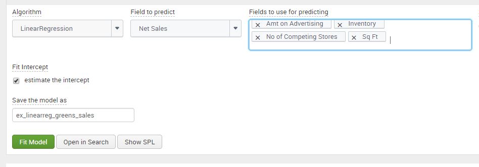
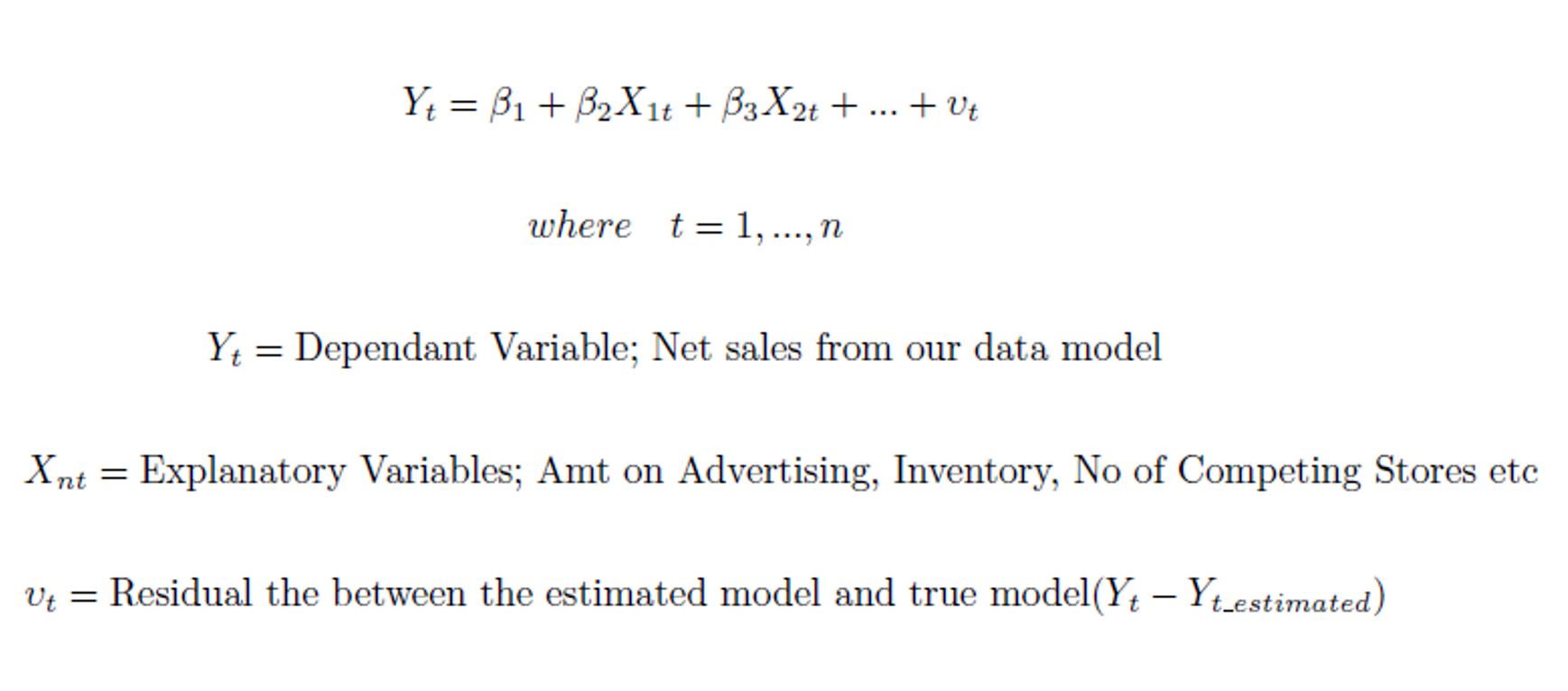
If you’re interested in the math behind it, linear regression from the Machine Learning Toolkit will provide us with the Beta (relationship) co-efficient between ‘Net Sales’ and each of the fields. The residual of regression model is the difference between the explanatory/input variables and the predicted equation at each data point, which can be used for further analysis of the model.
Fitting Model
Once the Fields have been picked, you need to determine the ‘Split for Training’ ratio for the model. Select ‘No Split’ for the model to use all the data for creating a model. The split option allows the user to divide the data for training and testing. This means that X% of the data will used to create our model, and (100-X) % of the data withheld will be used to test the model.
Click on ‘Fit Model’ after setting the Split for the data. Splunk processes the data to display visuals which we can use to analyze the data. Name the model ‘ex_linearreg_greens_sales’, however, based on the users data, the model name should reflect the field to predict, the type of algorithm and the user it is assigned to, to reduce ambiguity on the models ownership and purpose.
Analyzing the Results
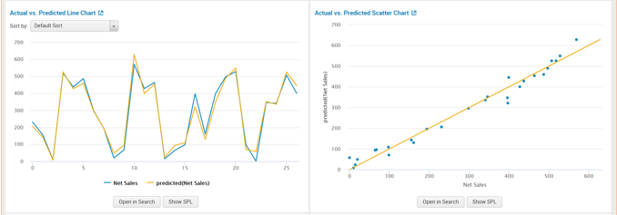
The first two panels show a Line and Scatter Chart of “Actual vs Predicted” data. Both panels present one of the richest methods to analyze the linear regression model. From the scatter and line plot we can observe that the data fits well. We can determine that there is a strong correlation between the model’s predictions and the actual results. Since the model has more than one input variable, examining the residual line chart and histogram next, will give us a more practical understanding.
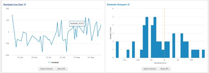
The second set of panels that we can use to analyse the model are residuals from the plot. From observing the “Residual Line Chart” and “Residual Histogram” we can see that there is large deviation from the center and the residuals appear to be scattered. A random scattering of the data points around the horizontal (x-axis) line signifies a good fit for the linear model. Otherwise, a pattern shape of the data points would indicate that a non-linear model from the MLTK should be used instead.
The last set of panels show us the R-squared of the model. The closer the value is to 1, better the fit of the regression model. The “Fit Model Parameters Summary” panel gives us the ‘Beta’ coefficients discussed in the ‘Selecting the Algorithm’ section. The assistant displays the data in a well-grounded and systematic setting. After analyzing the macro fit of the model, we can use the co-efficient of the variables create our equation for predicting ‘Net Sales’ :
In the last panel shown below, we can see our input variables under ‘Fit Model Parameters Summary’ and their values. We will assess in the next section on using these input variables to predict ‘Net_Sales‘.

Answering the Question: How is ‘Net Sales’ impacted by the Variables?
We can view the results of the model by running the following search:
| summary "ex_linearreg_greens_sales"
This Query will return the coefficients values of the linear regression algorithm. In our example for Greens, we observed that variable ‘X4’ are the number of competitors stores, an increment in competitors stores will reduce the ‘Net Sales‘ by approximately 12.62. While the variable ‘X5’ is the Sq Feet of the Store, and increment will increase the ‘Net Sales’ by approximately 23.69.
We can use the results from our model to forecast ‘Net Sales’ if the input variables (Sq Ft, Amt on Advertising etc) were different using the below Splunk search:
| makeresults | eval "Sq Ft"=5.8, Inventory=700, "Amt on Advertising"=11.5,"No of Competing Stores"=20 | apply ex_linearreg_greens_sales as "Predicted_Net_Sales"
We used makeresults to work our own values for the input variables. Once the fields have been defined we used the apply command in the MLTK to output the predicted value of the ‘Net Sales’ given the new values of the input variables. The apply command uses the ouput values the model learnt from the csv dataset and applies them to new information. We used the ‘as’ command to alias the name of the predicted field as ‘Predicted_Net_Sales’. From the below screenshot we can observe that; 11.5 on Advertising, 700 on Inventory, 20 Competing stores nearby and 5.8 square feet of space predicts a Net Sales of approximately 306. Please note that all monetary variables are in $1,000 .

Summary
So to recap, we followed the following steps to answer our question of the data:
- Uploaded the sample data set
- Populated the model fields
- Selected an algorithm
- Fit the model
- Analyzed the results
The Splunk Machine Learning Toolkit simplifies the steps for data preparation, reduces the steps needed to create a model, and saves the history of models we have executed and tested with. We can review the data before applying the algorithms allowing the user to standardize and adjust using MLTK capabilities or Splunk queries. The resulting statistic of the ‘Predict Numeric Fields’ assistant allows us to understand the dataset using machine learning.
Looking to expedite your success with Splunk? Click here to view our Splunk service offerings.
© Discovered Intelligence Inc., 2018. Unauthorised use and/or duplication of this material without express and written permission from this site’s owner is strictly prohibited. Excerpts and links may be used, provided that full and clear credit is given to Discovered Intelligence, with appropriate and specific direction (i.e. a linked URL) to this original content.
References
Houghton Mifflin, Data Sets, http://college.cengage.com/mathematics/brase/understandable_statistics/7e/students/datasets/mlr/frames/frame.html