We are pleased to announce the release of Config Quest 3.0, which further enhances this popular and innovative application. The new release introduces a new ‘File Config Quest‘ dashboard, allowing users to navigate through the file systems all Splunk hosts remotely and to compare file listings against one another. This post will run through some of the features of this new enhancement.
https://discoveredintelligence.com/wp-content/uploads/2019/10/cq_logo_3.png170200Discovered Intelligencehttps://discoveredintelligence.com/wp-content/uploads/2013/12/DI-Logo1-300x137.pngDiscovered Intelligence2019-10-13 17:10:142022-10-31 15:33:13What’s New In Config Quest 3.0
Part II of the Forecasting Time Series blog provides a step by step guide for fitting an ARIMA model using Splunk’s Machine Learning Toolkit. ARIMA models can be used in a variety of business use cases. Here are a few examples of where we can use them:
Detecting anomalies and their impact on the data
Predicting seasonal patterns in sales/revenue
Streamline short-term forecasting by determine confidence intervals
From Part 1 of the blog series, we identified how you can use Kalman Filter for forecasting. The observation we made from the resulting graphs demonstrated how it was also useful in reducing/filtering noise (which is how it gets its name ‘Filter’) . On the other hand ARIMA belongs to a different class of models. In comparison to a Kalman filter, ARIMA models works on data that has moving averages over time or where the value of a data point is linearly depending on its previous value(s). In these two scenarios it makes more sense to use ARIMA over Kalman Filter. However good judgement, understanding of the data-set and objective of forecasting should always be the primary method of determining the algorithm.
Objective
Part II of this blog series aims to familiarize a Splunk user using the MLTK Assistant for forecasting their time series data, particularly with the ARIMA option. This blog is intended as a guide in determining the parameters and steps to utilize ARIMA for your data. In fact, it is a generalized template that can be used with any processed data to forecasting with ARIMA in Splunk’s MLTK. An advantage of using Splunk for forecasting is its benefit in observing the raw data side by side with the predicted data and once the analysis is complete, a user can create alerts or other actions based on a future prediction. We will talk more about creating alerts based on predicted or forecasted data in a future blog (see what I predicted there ;)?)
If you have read part I of our blog, we will reuse the same dataset
process_time.csv
for this part. If not, click here to navigate to part I to understand the dataset.
Fundamental Concept for ARIMA Forecasting
A fundamental concept to understand before we move ahead with ARIMA is that the model works best with stationary data. Stationary data has a constant trend that does not change overtime. The average value is also independent of time as another characteristic of stationary data.
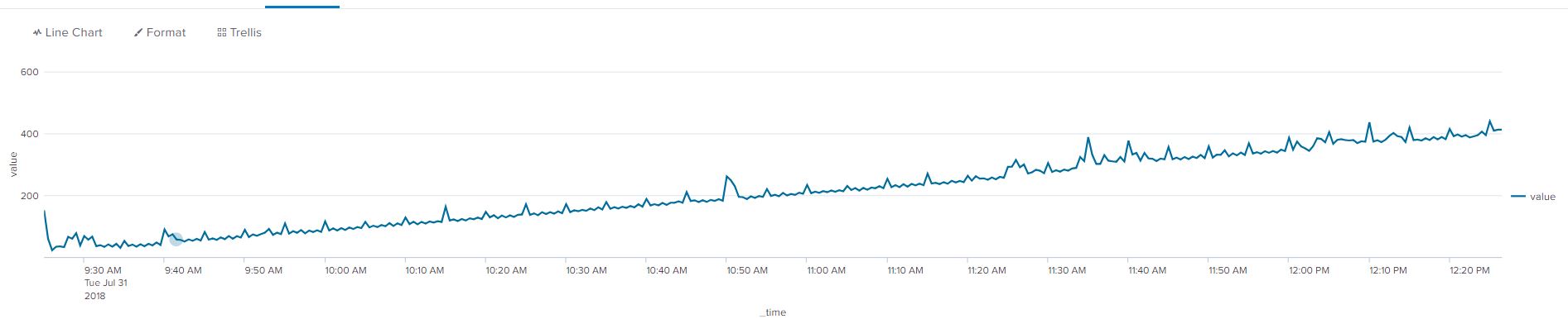
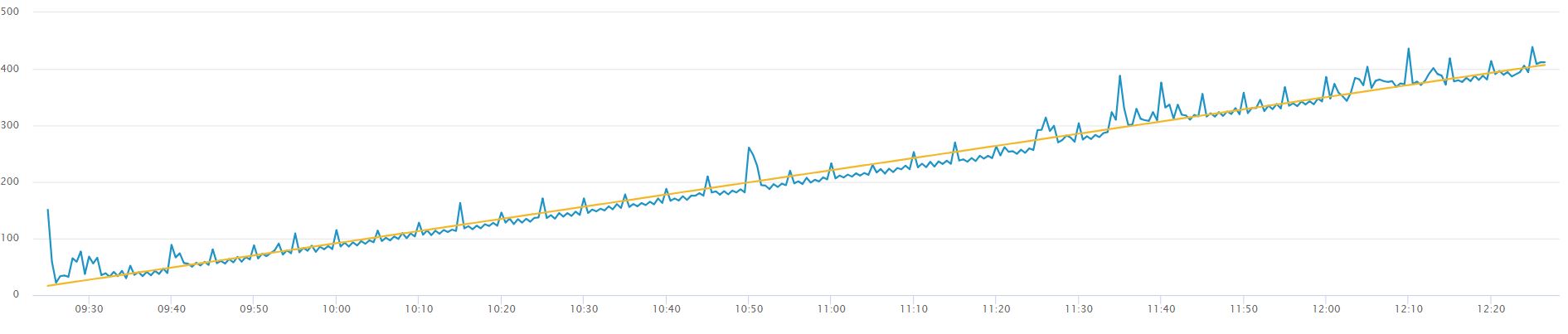
A simple example of non-stationary data is are the two graphs below, the first without a trendline, the second with a yellow trendline to show an average increase in the value of our data points. The data needs to be transformed into stationary data to remove the increasing trend.
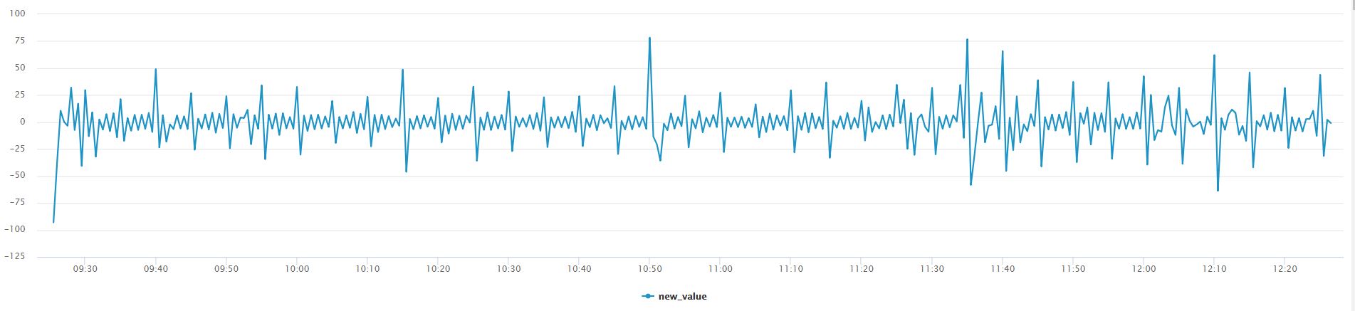
Using Splunk’s autoregress command we can apply differencing to our data. The results are immediately visible through line chart visual! The below command can be used on any time series data set to demonstrate differencing.
Without creating a trendline for the below graph we can see that the data fluctuates around a constant mean value of ‘0’, we can say that differencing is applied. Differencing to make the data stationary can increase the accuracy and fit of our ARIMA forecast. To read more about differencing and other rules that apply on ARIMA, navigate to the Duke URL provided in the useful link section:
Differencing is simply subtracting the current and previous data points. In our example we are only applying differencing by an order of 1, meaning we will subtract the present data point by one data point in reverse chronological order. There are different types of non-stationary graphs, which require in-depth domain knowledge of ARIMA, however we simplify it in this blog and use differencing to remove the non-constant trend in this example 😊!
From part 1 of this blog series we can see that our data does not have a constant trend, as a result we apply differencing to our dataset. The step to apply differencing from the MLTK Assistant is detailed in the ‘Determining Starting Points’ section. Differencing in ARIMA allows the user to see spikes or drops (outliers) in a different perspective in comparison to Kalman Filter.
Walkthrough of MLTK Assistant for ARIMA
ARIMA is a popular and robust method of forecasting long-term data. From blog 1 we can describe Kalman Filter’s forecasting capabilities as extending the existing pattern/spikes, sort of a copy-paste method which may be advantageous when forecasting short-term data. ARIMA has an advantage in predicting data points when the we are uncertain about the future trend of the data points in the long-term. Now that we have got you excited about ARIMA, lets see how we can use it in Splunk’s MLTK!
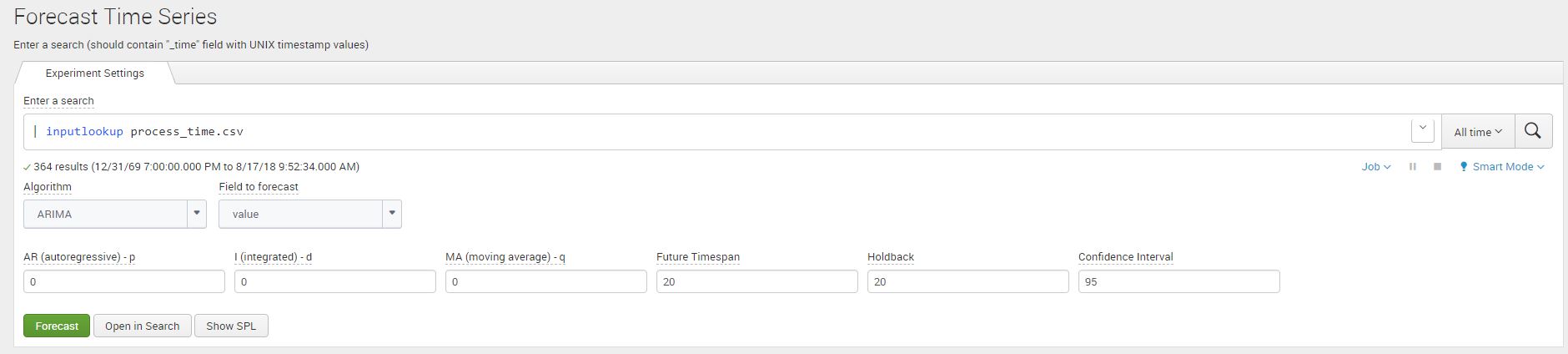
We use the Machine Learning Toolkit Assistant for forecasting timeseries data in Splunk. Navigate to the Forecast Time Series Assistant page (Under the Classic Menu option) and use the Splunk ‘inputlookup’ command to view the process_time.csv file.
|inputlookup process_time.csv
Once we add the dataset click on Algorithm and select ‘ARIMA’ (Autoregressive Integrated Moving Average), and ‘value’ as your field to forecast. You will notice that the ARIMA arguments will appear.
There are three arguments that make up the ARIMA model:
Argument
Definition
AutoRegressive – p
Auto regressive (AR) component refers to the use of past values in the regression equation. Higher the value the more past terms you will use in the equation. This concept is also called ‘lags’. Another way of describing this concept is if the value your data point is depending on its previous value e.g process time right now will depend on the process time 30 seconds before (from our data set)
Integrated – d
The d represents the degrees of differencing as discussed in the previous section. This makes up the integrated component of the ARIMA model and is needed for the stationary assumption of the data.
Moving Average – q
Moving Average in ARIMA refers to the use of past errors in the equation. It is the use of lagging (like AR) but for the error terms.
Determine Starting Points
Identify the Order of Differencing (d)
As a refresher, we utilized the same dataset we worked with in part 1 of the blog series regarding the Kalman filter. As I input my process_time.csv file in the assistant, I enter the future_timespan variable as 20 and the holdback as 20. I’ve kept the confidence interval as default value ‘95’. Once the argument values are populated click on ‘Forecast’ to see the resulting graphs.
As a note, my ARIMA arguments described above are ARIMA(0,0,0) which can represented as a mathematics function ARIMA(p,d,q), where p,d,q = 0. We use this functional representation of the variables frequently in this blog for consistently with generally used mathematical languages.
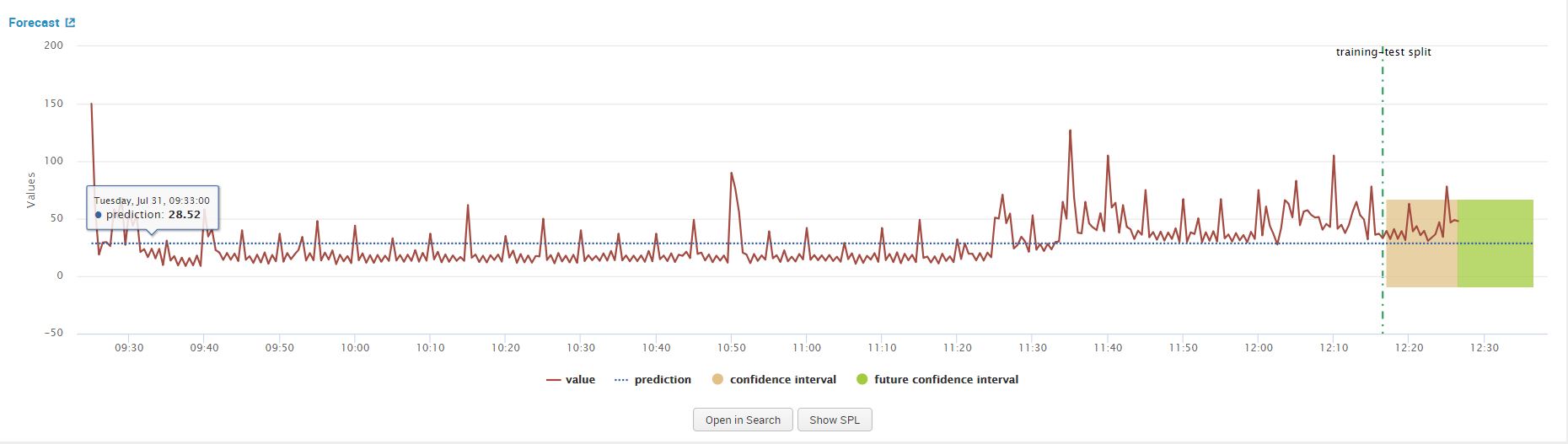
When we click on forecast, observe the line chart graph from the results that show. This above graph confirms that the data is non-stationary, we will apply differencing to make it stationary. We can accomplish this by increasing the value of our ‘d’ argument from ‘0’ to ‘1’ in the forecasting assistant and clicking on forecast again. This step is essential to meet one of the main criteria’s of using ARIMA discussed in the ‘Fundamental Concept for ARIMA’ section.
Identifying AR(p) and MA(q)
After we apply differencing to our data our next step is to determine the AR or MR terms that mitigate any auto correlation in our data. There are two popular methods of estimating the these two parameters. We will expand on one of the methods in this blog.
Method 1
The first method for estimating the value of ‘p’ and ‘q’ is to use the Akaiki Information Criteria (AIC) and the Baysian Information Criteria (BIC), however using them is outside the scope of the blog as we will use a different method from the MLTK given the tools we have at hand. For the curious mind, the following blog contains detailed information on AIC and BIC to determine our ‘p’ and ‘q’ values:
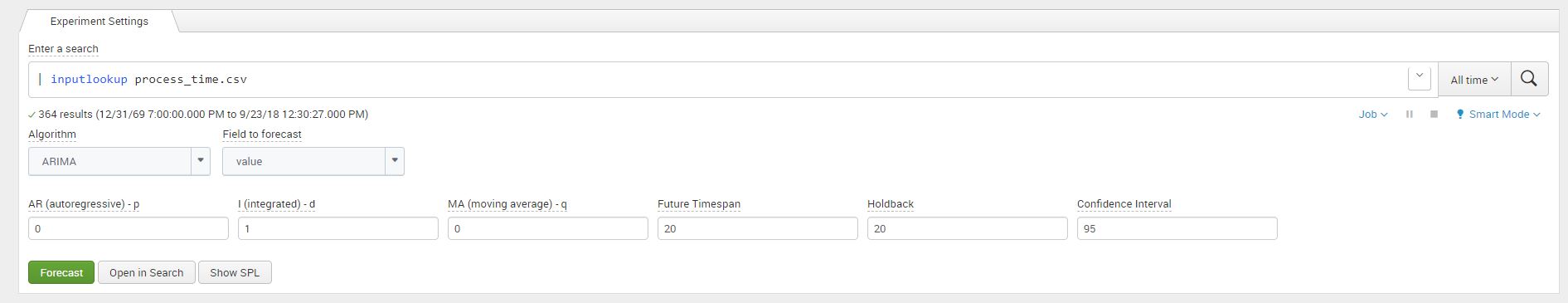
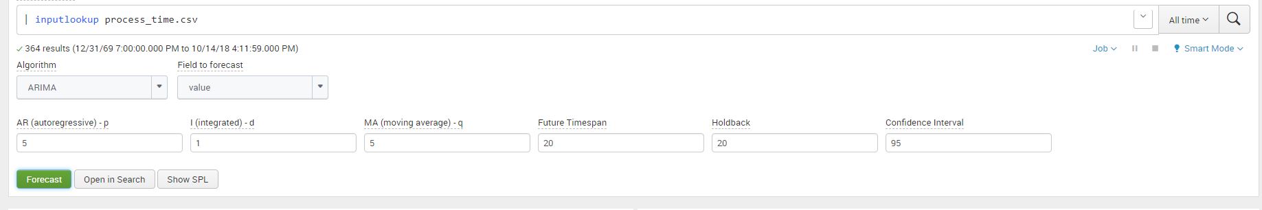
After we have applied differencing to our time series data, we review the PCAF and the ACF plots to determine an order for AR(q) or MA(q). We will apply ARIMA(0,1,0) in our ARIMA MLTK assistant and then click on ‘Forecast’ to view the results of the graph. The below image shows the values that we entered in the assistant:
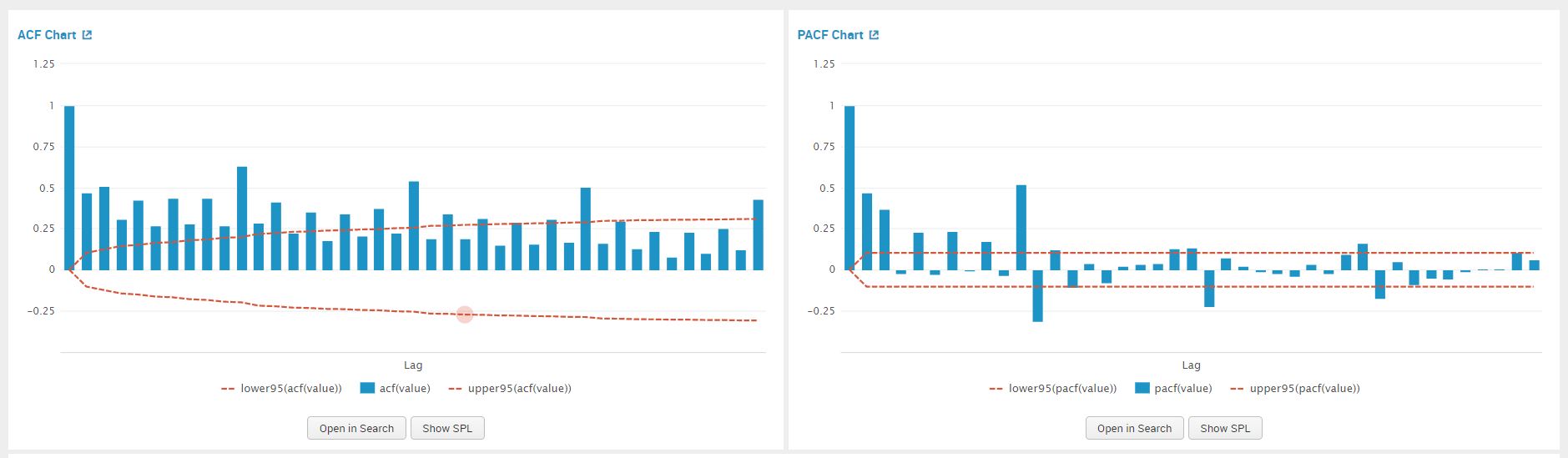
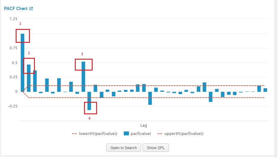
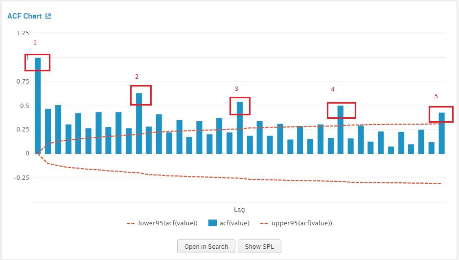
Once we click on forecast, we view the PACF plot to estimate a value for AR(p) model. Similarly we use the ACF plot to estimate a value for MA(q). The graphs are shown in the screenshot below.
We examine the PACF plot for a suggestion for our AR value, by counting the prominent high spikes. From the plot below I’ve circled the prominent spikes in the PACF graph. The value of AR (p) that we pick is 4.
We examine the ACF plot for a suggestion for our MA value, by counting the prominent high spikes. From the plot below I’ve circled the prominent spikes in the ACF graph. The value of AR (q) that we pick is 5.
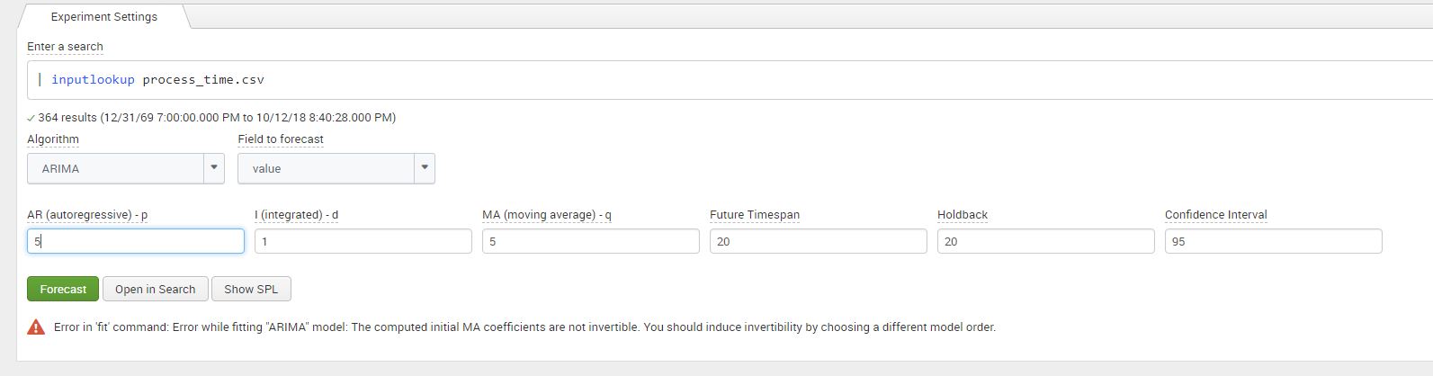
We can now add in the values for the parameter integrated (d) – 1 and our estimates for AR – 4, and MA -5 in the Splunk MLTK. Once added in the assistant, click on ‘Forecast’.
For this particular combination for values we can see that once we click on ‘Forecast’, we get an error regarding the ‘invertability’ of the dataset as shown in the screenshot below. Without going too deep into the mathematics, it means that our model does not converge when it forecasts. I’ve added a link in the references and links section at the end for your interest! This error can be resolved by adjusting the values of model, similar to a ‘trail an error’ approach explained in the next section.
Optimize Your P and Q Values
Estimating this method of AR and MA is subjective to what can be considered as ‘prominent spikes’, this can result in estimating values of ‘q’ and ‘p’ that are not an optimal fit for the data. To resolve this we constructed a table displaying the R-squared and Root Mean Square Error (RMSE) values from the model error statistics from the MLTK assistance, for each combination of ‘p’ and ‘q’. An empty cell indicates an invertability error, while the other cells contain the value of R-squared and RMSE.
A higher R-squared indicates a better fit the model has on the data. R-squared is the amount of variability that the model can explain on the process time data points.
On the other hand, the lower the RMSE is the better the fit of the model. Root mean square is the difference between the data points the model predicted and our holdback points from the raw data.
We pick values of ‘p’ and ‘q’ that minimize RMSE and maximize R-square as the best fit to our data. From the table below we can see that q=5 and p=5 optimize the prediction for us.
Integrated (d) = 0
AutoRegressive (p)
0
1
2
3
4
5
Moving Average (q)
0
R2 Stat: -0.0015
RMSE: 19.31
R2 Stat: 0.1976
RMSE: 16.35
R2 Stat: 0.1977
RMSE: 16.34
R2 Stat: 0.2699
RMSE: 15.60
R2 Stat: 0.2696
RMSE: 15.60
R2 Stat: 0.3114
RMSE: 15.14
1
R2 Stat: 0.2401
RMSE: 15.91
R2 Stat: 0.2486
RMSE: 15.82
R2 Stat: 0.2780
RMSE: 15.51
R2 Stat: 0.2329
RMSE: 15.98
–
R2 Stat: 0.4053
RMSE: 14.07
2
R2 Stat: 0.2452
RMSE: 15.85
–
–
R2 Stat: 0.3017
RMSE: 15.25
R2 Stat: 0.3214
RMSE: 15.03
–
3
R2 Stat: 0.2872
RMSE: 15.41
R2 Stat: 0.4185
RMSE: 13.92
R2 Stat: 0.4428
RMSE: 13.62
R2 Stat:
RMSE:
R2 Stat: 0.4343
RMSE: 13.72
R2 Stat: 0.4456
RMSE: 13.58
4
R2 Stat: 02826
RMSE: 15.46
R2 Stat: 0.4185
RMSE: 13.92
R2 Stat:0.3241
RMSE: 15.00
–
–
–
5
R2 Stat: 0.2826
RMSE: 15.46
R2 Stat: 0.3133
RMSE: 15.99
R2 Stat: 0.4385
RMSE: 13.67
–
–
R2 Stat: 0.4515
RMSE: 13.52
Viewing Your Results
Once we have picked the values of p and q that optimize our model, we can go ahead plug the numbers in our assistant and click on forecast to display the forecasted graph. The values to plug in the assistant are as follows: p-5, d-1, q-5, holdback-20, forecast-20. The screenshots below show the values entered in the assistant and the resulting forecast graph.
A this point many would be satisfied with the forecast as the visual of the data itself is enough to analyse, asses and then make a judgement on the action(s) to take. The next step details how you can view the data and lists some ideas of alerts that can be constructed
Next Step
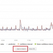
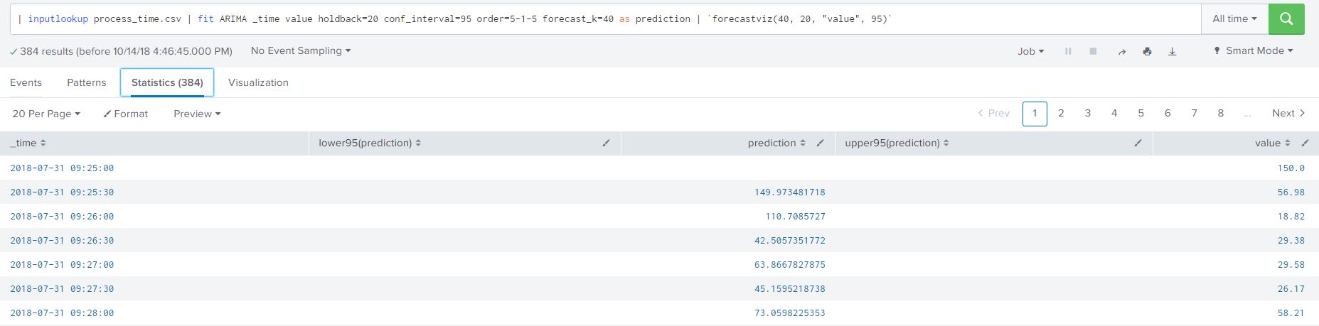
We can view the SPL used powering the graph by either clicking on ‘Open in Search’ or ‘ ‘Show SPL’. I prefer the ‘Open in Search’ option as it automatically open a new tab, allowing me to further understand how the SPL is constructed in the forecast and to view the data. Once a tab browser tab opens click on the ‘statistics’ option to view the raw data points, predicted data points and the confidence intervals created by our model. I have added the SPL from the image for your convenience below:
| inputlookup process_time.csv | fit ARIMA _time value holdback=20 conf_interval=95 order=5-1-5 forecast_k=40 as prediction | `forecastviz(40, 20, "value", 95)`
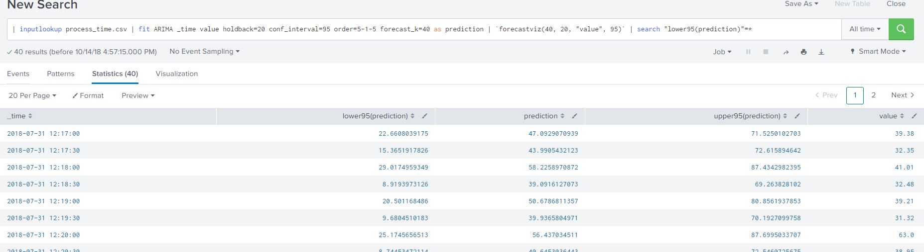
I added another filter to my SPL to only view the forecasted process data from the ARIMA model as shown below:
| inputlookup process_time.csv | fit ARIMA _time value holdback=20 conf_interval=95 order=5-1-5 forecast_k=40 as prediction | `forecastviz(40, 20, "value", 95)` | search "lower95(prediction)"=*
The resulting table lists all the necessary data in a clean tabular format (that we are all familiar with) for creating alerts based on our predicted process time. Here are some ideas on creating alerts based on the data we worked with:
Create alert when the predicted value of the process time goes above a certain threshold
Create alert when the average process time over a timespan is predict to stay above normal limits
Create alert based on outlier detection, when the predicted data is outside the lower or upper boundaries
Creating alerts based on our predict data allows us to be proactive of potential increase or decrease of our input variable
Summarizing ARIMA Forecasting in MLTK
Lets summarize what we have discussed so far in this blog:
A mathematical prerequisites of the model
Determining differencing requirement
Determine starting values for AR() and MA()
Optimize your AR() and MA() values based on error statistics
Forecast your data based on values decided in Step 4
View data and determine any alerts conditions
Prior to the above steps, we need to ensure that our data has been pre-processed or transformed in a MLTK-friendly manner. The pre-process steps include but not limited to; ensuring no gaps in the time series data, determine the relevance of data to forecasting, group data in time intervals (30 second, 1 minute etc). The pre-processing steps are important to create uniformity in the data input allow Splunk’s MLTK to analyse and forecast your data.
Hopefully this blog, streamlines the process of forecasting using ARIMA in Splunk’s MLTK. There are limitations as with any algorithm on forecasting using this method, as it involves a more theoretical knowledge in mathematics I’ve added two links in the the useful links section (first link is navigates you to on ‘datascienceplus.com’ and the second to ’emeraldinsight.com’) to further read on them.
https://discoveredintelligence.com/wp-content/uploads/2018/10/image-14.jpg5341823Discovered Intelligencehttps://discoveredintelligence.com/wp-content/uploads/2013/12/DI-Logo1-300x137.pngDiscovered Intelligence2019-05-06 12:21:352022-10-31 15:35:39Forecasting Time Series Data Using Splunk Machine Learning Toolkit – Part II
In early January of this year I was able to attend FloCon 2019 in New Orleans. In this posting, I will provide a little bit of insight into this security conference, some of the sessions that I attended, and detail some of the major data challenges facing security teams.
It was not hard to convince me to go to New Orleans for obvious reasons: the weather is far nicer than Toronto during the winter, cajun food and the chance to watch Anthony Davis play at the Smoothie King Center. I also decided to stay at a hotel off of Bourbon Street which happened to be a great decision. Others attending FloCon decided to arrange accommodations on Bourbon Street ended up needing ear plugs to get a good night’s rest! Enough about that though and let’s talk about the conference itself.
About FloCon
FloCon is geared towards researchers, developers, security experts and analysts looking for techniques to analyze and visualize data for protection and defense of networked systems. The conference is quite small, with a few hundred attendees rather than the 1000s that attend conferences I have attended in the past, like Splunk Conf and the MIT Sloan Conference. However, the smaller number of attendees in no way translated to a worse experience. FloCon was mostly single track (other than the first day), which meant I did not have to reserve my spot for popular session. The smaller number also resulted in greater audience participation.
The first day was split between two tracks: (1) How to be an Analyst and (2) BRO training. I chose to attend the “How to be an Analyst” track. For the first half of the day, participants of the Analyst track were given hypothetical situations which was followed by discussions on hypothesis testing and what kind of data would be of interest to an analyst in order to determine a positive threat. The hypothetical situation in this case was potential vote tampering (remember this is a hypothetical situation). The second half of the day was supposed to be a team game which involved questions and scoring based multiple choice answers. However, the game itself could not be scaled out to the number of participants, therefore the game was completed with all participants working together, which led to some interesting discussions. The game needs some work, but it was interesting to see how different participants thought through the scenarios and how individuals would go about investigating Indicators Of Compromise (IOCs).
The remaining three days saw different speakers present their research on machine learning, applying different algorithms to network traffic data, previous work experience as penetration testers, key performance indicators, etc. The most notable of the speakers being Jason Chan, VP of Cloud Security at Netflix. Despite some of the sessions being heavily research based and with a lot of graphs (some of which I’m sure went over the heads of some of us in attendance), common themes kept arising about the challenges faced by organizations – all of which Discovered Intelligence has encountered on projects. I have identified some of these challenges below.
Challenge: Lack of Data Standardization Breaks Algorithms
I think everyone knows that scrubbing data is a pain. It does not help that companies often change the log format with new releases of software. I have seen new versions break queries because a simple change has cascading effects on the logic built into the SIEM. Changing the way information is presented can also break machine learning algorithms, because the required inputs are no longer available.
Challenge: Under Investing in Fine-Tuning & Re-iterations
Organizations tend to underestimate the amount of time needed to fine-tune queries intended for threat hunting and anomaly detection. The first iteration of a query is rarely perfect and although it may trigger an IOC, analysts will start to realize there are exceptions and false positives. Therefore, overtime teams must fine-tune the original queries to be more accurate. The security team for the Bank of England spends approximately 80% of their time developing and fine-tuning use cases! The primary goal being to eliminate alert fatigue, and to keep everything up-to-date in an ever changing technological world. I do not think there is a team out there that gets “too few” security alerts. For most organizations, the reality is: that there are too many alerts and not enough resources to investigate. Since there are not enough resources, fine-tuning efforts never happen and analysts will begin to ignore alerts which trigger too often.
An example of the first iteration of an alert which can generate high volumes is failed authentications to a cloud infrastructure. If the organization utilizes AWS or Microsoft Cloud, they may see a huge number of authentication failures for their users. Why and how? Bad actors are able to identify sign-in names and emails from social media sites, such as LinkedIn or company websites. Given the frequently used standards, there is a good chance that bad actors can guess usernames just based off an individual’s first and last name. Can you stop bots from trying to access your Cloud environment? Unlikely, and if you could, the options are limited. After all, the whole point of Cloud is the ability to access it anywhere. All you can really do is minimize risk by requiring internal employees to use things like multi-factor authentication, biometric data or VPN. At least this way even if a password was obtained a bad actor will have difficulty with the next layer of security. In this type of situation though, alerting on failed authentications alone is not the best approach and creates a lot of noise. Instead, what teams might start to do is correlate authentication failures with users who do not have multi-factor enabled, thereby paying more attention to those who are at greater risk of a compromised account. These queries evolve through re-iteration and fine-turning, something which many organizations continue to under invest in.
Challenge: The Need to Understand Data & Prioritize
Before threats and anomalies can be detected accurately and efforts divided appropriately, teams have to understand their data. For example, if the organization uses multi-factor, how does that impact authentication logs? Which event codes are teams interested in for failed authentications on domain controllers? Is there a list of assets and identities, so teams can at least prioritize investigations for critical assets and personnel with privileged access?
A good example of the need to understand data is multi-factor and authentication events. Let’s say an individual is based out of Seattle and accessing AWS infrastructure requiring Okta multi-factor authentication. The first login attempt will come from an IP in Seattle, but the multi-factor authentication event is generated in Virginia. These two authentication events happen within seconds of each other. A SIEM may trigger an alert for this user because it is impossible for the user to be in both Seattle and Virginia in the given timeframe. Therefore, logic has to built in to the SIEM, so this type of activity is taken into consideration and teams are not alerted.
Challenge: The Security Analyst Skills Gap
Have you ever met an IT, security or dev ops team with too little work or spare time? I personally have not. Most of the time there is too much work and not enough of the right people. Without the right people, projects and tasks get prolonged. As a result, the costs and risks only rise overtime. Finding the right people is a common problem and not one just faced by the security industry, but there is a clearly a gap in the positions available and the skills in the workforce.
Challenge: Marketing Hype Has Taken Over
We hear the words all the time. Machine Learning. Artificial Intelligence. Data Scientists. How many true data scientists have you met? How many organizations are utilizing machine learning outside of manufacturing, telematics and smart buildings? Success stories are presented to us everywhere, but the amount of effort to get to that level of maturity is immense and there is still a lot of work to be done for high levels of automation to become the norm in the security realm.
In most cases, organizations are looking at data for the first time and leveraging new platforms for the first time. They still do not know what normal behaviour looks like in order to determine an event as an anomaly. Even then, how many organizations can efficiently go through a year’s worth of data to baseline behaviour? Do they have the processing power? Can it scale out to the entire organization? Although there is some success a turnkey solution really does not exist. Each organization is unique. It takes time, the right culture, roadmap planning and the right leadership to get to the next level.
Challenge: How Do You Centralize Logs? Understanding the Complete Picture
In order to accomplish sophisticated threat hunting and anomaly detection a number of different data sources must be correlated to understand the complete picture. These sources include AD logs, firewall logs, authentication, VPN, DHCP, network flow, etc. Many of these are high volume data sources so how will people analyze the information efficiently? Organizations have turned to SIEMs to accomplish this. Although SIEMs work well in smaller environments, scaling out appropriately is a significant challenge due to data volumes, a lack of resources (both people and infrastructure) and the lack of training and education for users and senior management.
In most cases, a security investigation begins and analysts start to realize there are missing pieces and missing data sets to get the complete picture of what is happening. At which point, additional data sources must be on-boarded and the fine-tuning process starts again.
Wrap Up and FloCon Presentations
This posting highlights some of the data challenges that are facing security teams today. These challenges are present in all industry verticals, but with the right people and direction companies can begin to mature and automate processes to identify threats and anomalies efficiently. Oh, and did I mention, with our industry leading, security data and Splunk expertise, Discovered Intelligence can help with this!
https://discoveredintelligence.com/wp-content/uploads/2019/04/flocon2019.png155360Discovered Intelligencehttps://discoveredintelligence.com/wp-content/uploads/2013/12/DI-Logo1-300x137.pngDiscovered Intelligence2019-04-25 19:18:182025-12-17 16:31:41FloCon 2019 and the Data Challenges Faced by Security Teams
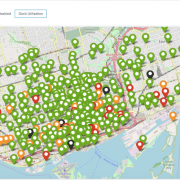
With the New Year, and cold winter, now upon us here in Toronto we thought it would be fun to kick it off by revisiting our award winning Hackathon entry from last years Splunk’s Partner Technical Symposium and adapting it to provide insights for our very own Toronto’s Bike Share platform leveraging their Open Data.
https://discoveredintelligence.com/wp-content/uploads/2018/10/Dock-Utilization.png499975Dhiren Meswaniahttps://discoveredintelligence.com/wp-content/uploads/2013/12/DI-Logo1-300x137.pngDhiren Meswania2019-01-11 17:09:492022-10-31 15:38:20Fun with Open Data: Splunking Bike Share Toronto