Are you tired of hardcoding email addresses into your searches and alerts? Do you want a more dynamic way to send search results to individuals based on the data within your search results? Look no further than SendResults, a powerful Splunk command and alert action developed by Discovered Intelligence.
https://discoveredintelligence.com/wp-content/uploads/2023/08/sendresults_command.png400600Discovered Intelligencehttps://discoveredintelligence.com/wp-content/uploads/2013/12/DI-Logo1-300x137.pngDiscovered Intelligence2023-08-09 14:55:212025-12-17 16:28:41Discover the Power of SendResults: A Life-Changing Splunk Command and Alert Action
If you haven’t heard of ChatGPT yet, you likely have blocked notifications on social networks like Linkedin, Twitter or Reddit, as everyone is talking about the benefits (and concerns) of artificial intelligence. However, it’s ChatGPT who gets the lion’s share of the limelight in this story.
https://discoveredintelligence.com/wp-content/uploads/2023/05/chatgpt_help.png353685Discovered Intelligencehttps://discoveredintelligence.com/wp-content/uploads/2013/12/DI-Logo1-300x137.pngDiscovered Intelligence2023-05-31 23:53:072023-06-01 13:53:05ChatGPT and SPL: A Dynamic Duo for Learning Splunk’s Query Language
Workload management is a powerful Splunk Enterprise feature for users to delegate CPU and memory resources to various Splunk workloads, based on their preferences. As Splunk continues to develop new attributes for the defining of rules, the number of Splunk users who are enabling workload management in their environment is gradually increasing.
The quote from Check Point Research above illustrates where the future trend of cybersecurity is headed and the challenges that organizations must face. However, anticipating and preparing the system defenses to evade and mitigate these attacks is not an easy task. From defining response and incident strategies to preparing work teams and configuring monitoring systems, it can all be a challenge.
Your core business is not to detect and mitigate security attacks, but is this essential to the achievement of your objectives? Have you ever wondered how you can simulate attacks and detections within a controlled environment to validate the configuration of your detection systems without spending part of your annual security budget? Read on and discover Splunk Attack Range.
What is Splunk Attack Range?
Splunk Attack Range is a tool developed by Splunk Threat Research Team (STRT) to simulate cyber attacks in a controlled environment for the purpose of improving an organization’s security posture. It allows security teams to test and validate their detection and response capabilities against a wide range of attack scenarios and techniques, such as phishing, malware infections, lateral movement, and data exfiltration.
Splunk Attack Range is designed to work with Splunk Enterprise Security, which is a security information and event management (SIEM) solution, and includes pre-built attack scenarios that are aligned with the MITRE ATT&CK framework, these ones can be customized to simulate the specific threats and vulnerabilities that are relevant to an organization’s environment.
Where can I get Attack Range?
The STRT and the Splunk community are maintaining the project in GitHub.
Is Splunk Attack Range Easy to Deploy?
Yes, it is really straightforward! You can deploy it locally (if you have a powerful machine), on Azure or on AWS. Internally, we use our AWS environment and with a few simple steps, in a matter of minutes, terraform and ansible automatically deploy a complete test lab to validate our customers’ security configurations and optimize the security posture with Splunk’s real-time monitoring. This process allows for a proactive approach to managing security postures with Splunk and saves a lot of time for your Blue Team.
…and now?
Have fun! By merging our Splunk expertise and using these kinds of automation tools, we have been able to speed up our internal testing processes, stay agile and secure with Splunk’s security posture management tool, and transfer this knowledge and configurations on to our customers’ cybersecurity teams.
We strongly encourage you to try this tool. Check out an overview of v1.0, v2.0 and v3.0 in the Splunk blog.
https://discoveredintelligence.com/wp-content/uploads/2023/03/splunk-attack-range-logo-e1678466676167.png693696Discovered Intelligencehttps://discoveredintelligence.com/wp-content/uploads/2013/12/DI-Logo1-300x137.pngDiscovered Intelligence2023-03-14 15:17:262023-03-14 15:17:29Save Time and Improve your Security Posture with Splunk Attack Range
Once you have embraced and grasped the power of Cribl Stream, “Reduce! Simplify!” will become your new mantra.
Here we list some of the best Cribl Stream resources available to get you started. Most of these resources are completely free! – money is not an obstacle when beginning your Cribl Stream journey, so keep reading and start learning today!
https://discoveredintelligence.com/wp-content/uploads/2023/02/getting_started_with_cribl.png582550Terry Mulliganhttps://discoveredintelligence.com/wp-content/uploads/2013/12/DI-Logo1-300x137.pngTerry Mulligan2023-02-23 15:20:382024-01-19 02:44:06Help Getting Started with Cribl Stream
Deploying apps to forwarders using the Deployment Server is a pretty commonplace use case and is well documented in Splunk Docs. However, it is possible to take this a step further and use it for distribution of apps to the staging directories of management components like cluster manager or a search head cluster deployer, from where apps can then be pushed out to clustered indexers or search heads.
Planning a sequel to the blog –Moving bits around: Deploying Splunk Apps with Github Actions – led me to an interesting experiment. What if we could manage and automate the deployment server the same way, without having to log on to the server at all. After all, the deployment server is just a bunch of app directories and a serverclass.conf file.
In our previous blog we covered some common methods of finding an outliers. Starting with fixed thresholds to moving thresholds using averages and standard deviation. This forms the basis of data points that deviate from their norm. Using standard methods of outlier detection does have it pro’s and con’s. On one hand they are very easy to implement and derive reason for outlier detection. On the other hand, they are too simple
Key Concepts In this Blog
The terminology we will use will not differ significantly from our previous blog except with the introduction of the following terms:
Density Function Command: The density function command is housed within the MLTK application. Most mathematicians think about Z-score or normal distribution when a density function is mentioned. However within Splunk’s MLTK command there are 4 distributions that attempt to map the distribution of the data. They are ‘Normal (Z-score), Exponential, Gaussian Kernel Density and Beta Distribution’. The command will attempt to find the best distribution fit for the data given the split-by field.
More can be read about this command the Splunk blog post here.
Ensemble Methods: Ensemble methods is a technique within the Machine Learning space to combine multiple algorithms to create an optimal model. My favourite blog channel ‘towards data science’ explains it here.
Using MLTK Algorithms for Outlier Detection
Splunk’s Machine Learning Toolkit hosts 3 algorithms for anomaly detection. Whilst they each provide value, some may better suited in specific scenarios. Most if not all of the anomaly detection algorithms can be used on numerical and categorical fields. To illustrate their feature we picked the Density Function to enumerate and deep-dive into here.
DensityFunction
The density function is a popular and relatively simple method of finding outliers assuming no changes to default parameters. Underneath the hood though, it contains many configuration opens for users to fine tune their outlier detection. Lets cover some of the parameters I’ve come across tuning in the field:
parameter
default_value
description
when to adjust parameter
sample
false
When set to true, it takes sample from the ‘inliear’ region of the distribution.
When you have a large volume of data points + and need to remove initial outliers from your model. This is beneficial when you have more than a million events as the density function has a soft limit on events.
full_sample
false
When set to ‘true’ it takes sample from the ‘inliear’ and ‘outlier’ region of the distribution.
When you have a large volume of data points and would like to consider outliers samples in your outlier detection model. This is beneficial when you have more than a million events as the density function has a soft limit on events.
dest
auto
When set to ‘true’ the density of each data point will show.
Our suggestion is keep this as ‘auto’ . It allow MLTK to determine the best algorithm based on the values of each group. Set this as a specific distribution when the distribution is expected to a singular.
random_state
N/A
Identify which distribution you should like to run.
Use this parameter when developing your model on a fixed data set. Using the same random_state with all other configurations unchanged will return the same result. This is helpful to use when two or more users are working off the same data.
partial_fit
false
Incrementally ‘train’ and update the model based on new data. This is useful when you have a large volume of data and are unable to train.
Scenarios where using partial fit is helpful is to train your function over time where running a single fit command will reach an MLTK limit; such as over 7 days, 1 month and so on.
threshold
0.01
1 less than the threshold value shows the area under the curve.
This parameter can be adjusted to ease or restrict the criteria for detecting outliers. The smaller the value the less number of outliers (more restrictive) will be. On
List of commonly used parameters from Density Function
Adding onto a list of useful parameters, there is a ‘by’ clause within the Density Function. It gives the user the ability to group data based on a categorial field (grouping field). This grouping field can be location, intranet zone, host type, asset type, user type and much more. Lets start building some searches to utilize the density function:
Base Query
The base query to understand the Density Function a bit better is shown below. We are using the out-of-the-box lookup to run our query. The file ‘call_center.csv’ contains a list of call records count over a 2 month period starting in September 2017 till November. Next we are running 2 eval functions to extract the HourOfDay and DayOfWeek from the data.
Univariate in this context means that we will analyze outliers based on a single field of interest. For this section we picked ‘DayOfWeek’ as the field. We appended any new queries to our base query. This search will run the density function on the total count of activity based on the DayOfTheWeek. It will give us list of outliers, boundary range the outlier fill in and the probability density of the outlier. The two columns to focus on are “IsOutlier(count)” and “ProbabilityDensity(count)”. The lower the probability density, the higher the chance the value of count on the DayOfTheWeek has to be an outlier.
... | fit DensityFunction count by DayOfWeek into densityfunction_testmodel
Once we run the fit command, we can see 3 new columns created named “isOutlier(count), BoundaryRanges, ProbabilityDensity(count)”.
Using the density function is quite simple as using the fit command provided by MLTK. In order to use the DensityFunction algorithm effectively I will recommend to test and verify outliers with different parameters configurations. One such parameter that you can modify is the ‘threshold’ function. To test its impact on the result, I created a table below to analyze the outlier count based on different values.
Threshold
Outlier Count ‘(| stats count(eval(is_outlier=1)) as outlier_count’
0.01 (default)
116
0.05
590
0.09
1027
0.005
59
0.001
11
Table displaying outlier count on varied thresholds
After creating the table, it becomes clear as the thresholds value decreases, the DensityFunction is more restrictive in finding outliers. As we increase the threshold value outliers number increase as it becomes less restrictive.
Visualizing Changing Parameters with DensityFunction
To visual the impact of the different threshold levels we add the ‘show_option’ parameters to the density function as shown below:
... | fit DensityFunction count by DayOfWeek into densityfunction_testmodel threshold=0.005 show_density=true show_options="feature_variables, split_by, params"
After that, we use the MLTK ‘distribution plot’ visual to look at the distribution plot of the data.
Distribution Plot of All Days of Week
From the above plot, each line represents each day of the week, Monday thru Sunday. However, to view this with clarity lets filter this visual to a single day only in the picture below.
... | fit DensityFunction count by DayOfWeek into densityfunction_testmodel threshold=0.005 show_density=true show_options="feature_variables, split_by, params"
| search DayOfWeek="Monday"
Distribution Plot of Monday Only
In the above distribution plot, we can see that on Monday, the call volumes of around 900, 1100 1250 and 1300 were detected as outliers. It might appear that the outliers exist on the right side of the graph because they are extremely high values compared to the rest of the calls volumes. However, they are detected as outliers due to the low probability of these high values occurring.
Looking at the same Distribution Plot of Monday, the range of values between 300-500 have a low count as well. As we increase the thresholds we to 0.05. Notice how more values with low counts will be selected. This is due to the lower probability of them occurring in the dataset of and us relaxing the threshold. This concept ties back directly to the table we built in the ‘Using The Density Function - Univariate Outlier‘ section.
... | fit DensityFunction count by DayOfWeek into densityfunction_testmodel threshold=0.05 show_density=true show_options="feature_variables, split_by, params"
| search DayOfWeek="Monday"
Distribution Plot of Monday with Threshold=0.05
Conclusion
The DensityFunction is great and easy to use algorithm available along with MLTK for finding outliers. It’s very well documented in the Splunk Documentations and used commonly in the community. Some of the scenarios I’ve found it to be helpful in are listed below:
Quick and easy scenario’s use of ML to find outliers
Use cases where anomalies in aggregate counts are used to find outliers
Finding unexpected counts over times and hours when activity counts are not expected
However, one drawback and feature to using the DensityFunction is that it does not have historic or outside context. It will find outliers based on counts and its deviations. This can result in a same entities selected as outliers in multiple iterations over multiples times. One of the ways to tackle this is via adding context and using scores in Splunk. We talk about this method in our blog https://discoveredintelligence.ca/reducing-outlier-noise-in-splunk/.
https://discoveredintelligence.com/wp-content/uploads/2013/12/DI-Logo1-300x137.png00Discovered Intelligencehttps://discoveredintelligence.com/wp-content/uploads/2013/12/DI-Logo1-300x137.pngDiscovered Intelligence2022-02-14 15:44:062024-07-28 15:19:17Using DensityFunction for Outlier Detection in Splunk
The Splunk Machine Learning Toolkit is packed with machine learning algorithms, new visualizations, web assistant and much more. This blog sheds light on some features and commands in Splunk Machine Learning Toolkit (MLTK) or Core Splunk Enterprise that are lesser known and will assist you in various steps of your model creation or development. With each new release of the Splunk or Splunk MLTK a catalog of new commands are available. I attempt to highlight commands that have helped in some data science or analytical use-cases in this blog.
https://discoveredintelligence.com/wp-content/uploads/2020/10/image-10.png2561892Discovered Intelligencehttps://discoveredintelligence.com/wp-content/uploads/2013/12/DI-Logo1-300x137.pngDiscovered Intelligence2020-11-12 20:24:382022-10-31 14:41:21Interesting Splunk MLTK Features for Machine Learning (ML) Development
Recently a customer was reviewing information in Splunk and some interesting data showed up. Users had mobile devices that had emoji’s in their name of their device.
It was a bit surprising at first as it’s not what you would normally expect in a corporate IT environment, but after thinking about it, it’s perfectly normal to see – especially with companies fully adopting BYOD programs these days.
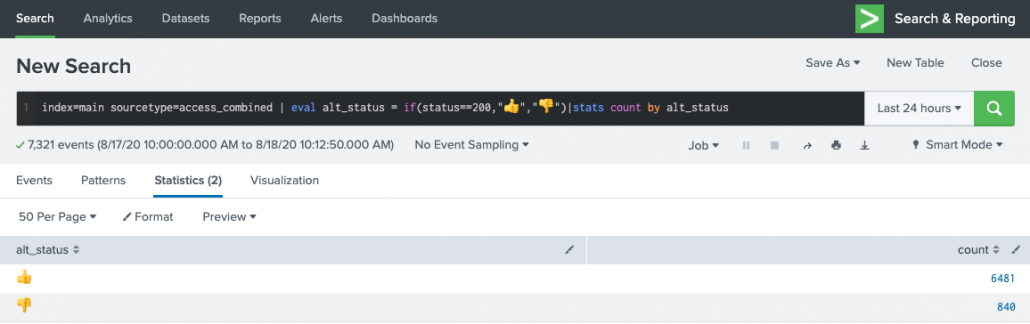
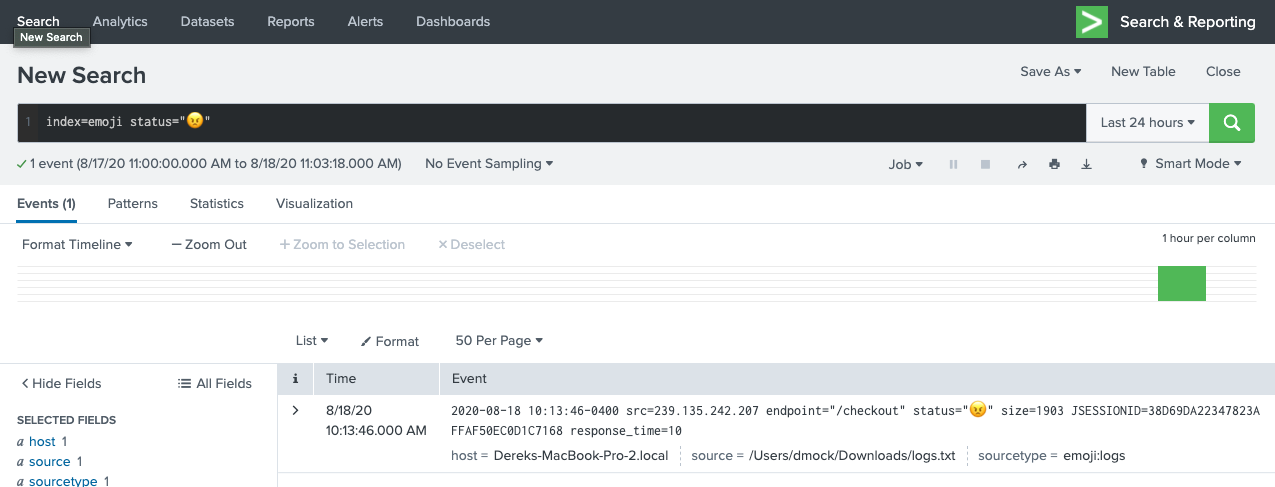
If you weren’t already aware, Splunk can handle different character sets. You can work with non-ascii characters in various different ways – including emojis! From indexing data, searches, alerts, and dashboards. Once you get into the world of non-ascii, you are dealing with Unicode. Unicode is a complex topic. There are many different concepts and terminology to keep straight. But that’s not really the point of this blog 😉 . For more information on Unicode you can start here.
It certainly gets you thinking 🤔 , where could emojis be used in Splunk to inject a bit of fun. Why not give your searches and Splunk dashboards a little ❤️ ?
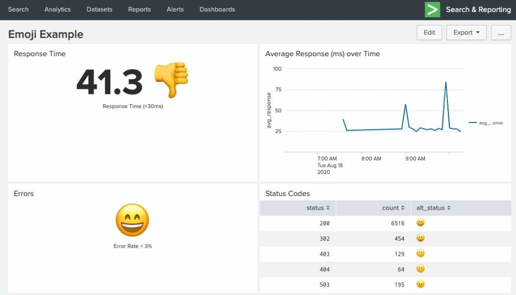
Errors single-value panel: index=main sourcetype=access_combined | stats count(eval(status >= 500)) as errors count as total | eval error_rate=round((errors/total)*100,1) | eval alt_status = if(error_rate >= 3, "😕","😄")| fields alt_status
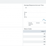
Status Codes table panel: index=main sourcetype=access_combined | stats count by status | eval alt_status = case(status >= 500, "😠",status >=400, "😕", status >= 200, "😄", 1==1,"❓")
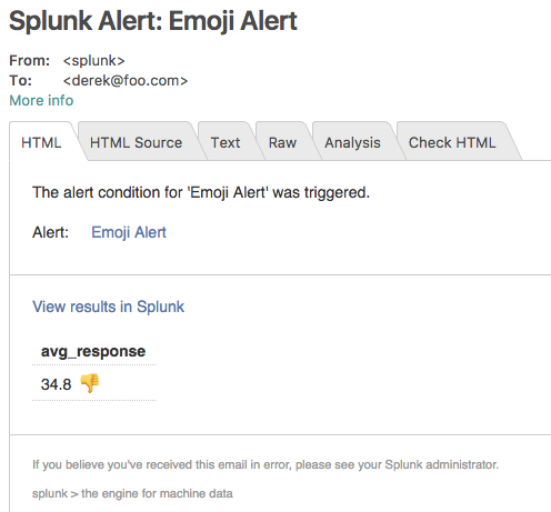
Or even using them in alerts (results will vary depending if the target of the alert can handle Unicode). Here’s an email example with the results embedded inline:
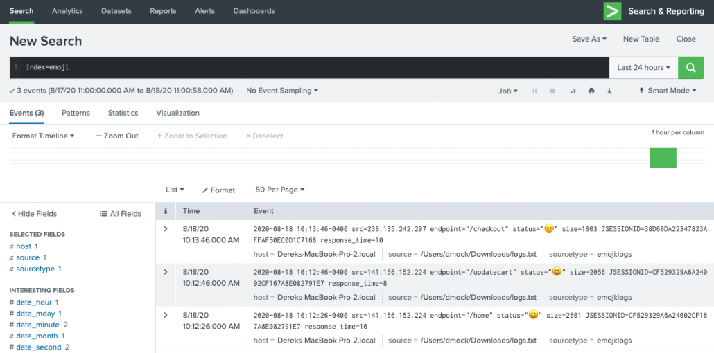
Maybe you can live on the wild side and even ask your developers to start using emoji’s in their logs….
Ok, that’s fun and all, but is there a practical use for emoji’s in Splunk? Sure! Why not give your dashboards some more visual eye candy when it comes to location data. You can easily create a lookup that maps Country name to their emoji flag.
Top Country single-value panel: index=main sourcetype="access_combined" | top limit=1 clientip | iplocation clientip | eval Country = if(Country=="", "Unknown", Country) | lookup emoji_flags name as Country OUTPUT emoji | fillnull value="❓" emoji | eval top_country= Country." ".emoji | fields top_country
Requests By Country table panel: index=main sourcetype="access_combined" | stats count by clientip | iplocation clientip | eval Country = if(Country=="", "Unknown", Country) | stats sum(count) as total by Country | lookup emoji_flags name as Country OUTPUT emoji | fillnull value="❓" emoji | sort - total
You can download the flag to emoji lookup CSV here to use in your own searches.
The possibilities are endless! So have some fun with emojis in your dashboards, lets just hope that at no point do your dashboards or data go to 💩 …